How to explain the behavior of vision transformers?
This page's goal is to present techniques that can shed light on how Vision Transformers' models (ViTs) operate. We will first have a refresher on the ViTs and how they work. We will develop a simple ViT classifier trained on the 🐶🐱 dataset and use a pre-trained model to efficiently classify the images. The next step is to introduce various methods to visualize the way that the classifier makes specific decisions. These approaches range from visualizing the attention maps to visualizing the query/key and value, but also using the backpropagated gradient similar to gradCAM algorithm. We will make use of PyTorch implementation to demonstrate some of these techniques. At the end of the blog post, there is a simple assignment TODO that you will need to solve as homework.
Introduction
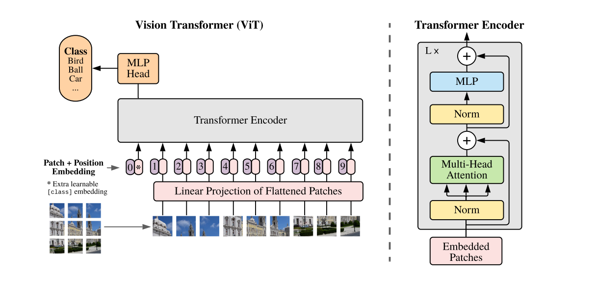
Fig 1. Vision transformer architecture. In the left part, we can see the whole framework, from the patch calculation, patch embeddings, the positional encoding, transformer encoder and the classifcation head. While in the right part we can see the Encoder architecture.
So what is a Vision Transformer? What is going on with the inner parameters of it? How do they even work? Can we poke at these parameters and dissect them into pieces to understand them better? These are some fundamental questions that we will try to answer in this post.
- Firstly, we will try to remind our reader about what is exactly a vision transformer and how it works.
- We will develop a simple image classifier that distinguishes between 🐶🐱 images. Moreover, we will try to showcase methods that aim to shed light on the inner mechanisms of the
ViTmodel. - We will make use of
PyTorchto implement these methods and showcase the results. Moreover, we will make use of two different XAI methods. - Finally, a simple TODO exercise will be provided to gauge the performance of different XAI methods for our built
ViTmodel.
Vision Transformer ViT
The vanilla Transformer architecture was introduced by Vaswani et al. in 2017 [1], to tackle sequential data and particularly textual information for the machine translation task. Given the success of the Transformer in the NLP domain, Dosovitskiy et al. [2] proposed the Vision Transformer (ViT) architecture for visual classification tasks. The ViT architecture is the standard transformer architecture but with visual information as input instead. In the ViT context, we need to convert the grid of pixels into a sequence of token embeddings. This could be done by splitting the image into non-overlapping patches and then, each patch should be flattened into a 1D vector and then linearly projected into a vector of token embeddings. Finally, these token embeddings are fed into the ViT architecture in a similar way as the vanilla transformers.
The basic blocks of the ViT architecture can be seen in the previous image and are:
- Patch + Position Embedding: Turns the input image into a sequence of image patches and adds a position number to specify in what order the patch comes in.
- Embedded Patches: The image patches are flattened and then projected into embeddings. The benefit of using embeddings rather than just the image values is that embeddings are learnable representations of the image that can improve with training.
-
Transformer Encoder: The Transformer Encoder, is a collection of the layers listed above. There are two skip connections inside the Transformer encoder (as they are portrayed in the Architecture image) meaning the layer’s inputs are fed directly to immediate layers as well as subsequent layers. The overall
ViTarchitecture is comprised of several Transformer encoders stacked on top of each other.-
Layer Normalization: This is short for
Layer NormalizationorLayerNorm, a technique for regularizing (reducing overfitting) a neural network, you can use LayerNorm via thePyTorchlayertorch.nn.LayerNorm(). -
-
Multi-Head Attention: This is a Multi-Headed Self-Attention layer or
MSAfor short. You can create an MSA layer via the PyTorch layertorch.nn.MultiheadAttention().
-
Multi-Head Attention: This is a Multi-Headed Self-Attention layer or
-
MLP (or Multilayer perceptron): An MLP can often refer to any collection of feedforward layers (or in PyTorch’s case, a collection of layers with a forward() method). In the
ViTPaper, the authors refer to the MLP as “MLP block” and it contains twotorch.nn.Linear()layers with atorch.nn.GELU()non-linearity activation in between them (section 3.1) and atorch.nn.Dropout()layer after each.
-
Layer Normalization: This is short for
- Classification Token: Similar to BERT architecture a classification token is added to the input sequence. We will use the output feature vector of the classification token (CLS token in short) for determining the classification prediction.
-
MLP Head: This is the output layer of the architecture, it converts the learned features of an input to a class output. Since we’re working on image classification, you could also call this the “classifier head”. The structure of the
MLPHead is similar to the MLP block. - Output predictions
To help the reader comprehend all the above, we will provide a simple grouping of definitions and use the following two terms:
- layers: are basic elements that are used to build the architecture. For example, the multi-head self-attention can be considered as a layer. It’s important to mention that a Transformer is composed usually of several Encoders. Each of these Enconders can be referred to in the literature as a layer as well.
- blocks: a grouping of layers (for instance the whole encoder can be seen as a block of layers).
Finally, a list with all the hyperparameters that we will need to define for the ViT model is as follows:
- Layers: How many Transformer Encoder blocks are there? (each of these will contain an MSA block and the MLP block)
- Hidden size D: This is the embedding dimension throughout the architecture, this will be the size of the vector that our image gets turned into when it gets patched and embedded. Generally, the larger the embedding dimension, the more information can be captured, which leads to better results. However, a larger embedding comes at the cost of more computing. One niche issue here is that we need to distinguish the layers as hyperparameters that refer to the number of Transformer Encoder blocks and the layer as a building block of the encoder.
- MLP size: What are the number of hidden units in the MLP layers?
- Heads: How many heads are there in the Multi-Head Attention layers?
Vision Transformers (ViTs) Tokenization
The standard Transformer receives as input a 1D sequence of token embeddings. To handle 3D images, we reshape the image $\mathbf{x} \in \mathbb{R}^{H \times W \times C}$ into a sequence of flattened patches with size $\mathbf{x}_{P} \in \mathbb{R}^{N \times CP^2}$, when $H, W$ represent the height and the width of an image while $C$ represents the number of channels, then, $N$ is the number of patches and $P$ is the patch dimensionality. The Transformer uses constant latent vector size $D$ through all of its layers, so we flatten the patches and map them to $D$ dimensions with a trainable linear projection (Equation 1 from the ViT paper). This projection can be referred to as patch embeddings. If the input image is of size $224 \times 224 \times 3$ and the patch size is $16$ then the output should be of size $196 \times 768$ ($196 = 14 \times 14$), where the first dimension is the number of patches and the second dimension is the size of the patch embeddings $16\cdot 16\cdot 3 = 768$.
Positional encoding
In the same spirit, with the vanilla Transformer architecture, we will need to ensure that the architecture is always aware of the position of the patches. This is done by adding a positional encoding. It is a learnable parameter that is added to the patch embeddings. It is represented as a matrix of size $N \times D$ where $N$ is the number of patches and $D$ is the size of the patch embeddings. Then it is added to the patch embeddings before they are fed into the Transformer Encoder blocks. Since we usually work with a fixed resolution, we can learn the positional encodings instead of having the pattern of sine and cosine functions.
Transformer enconder
After having created the patches, we should proceed with the implementation of the transformer encoder which can be seen in the above Figure. It can mainly divided into the multi-head attention (MSA) and the MLP layer. The multi-head self-attention mechanism is used to capture the dependencies between the patches. The feed-forward neural network is used to capture the non-linear interactions between the patches. The following image portrays the mechanism of the attention block. Here we will need to decide whether the input to our model will be the full image or the image patches. To decide that we will take into account that a lot of pre-trained models have as input the full image. Thus, for now, we will use the full image as input to our model.
More info and more details about the transformer encoder can be found in the original ViT paper.
Fig 2. Vision transformer architecture. In the left part, we can see the whole framework, from the patch calculation, patch embeddings, the positional encoding, transformer encoder and the classifcation head. While in the right part, we can see the Encoder architecture.
Layer normalization
Inspired by the results of Batch Normalization, Geoffrey Hinton et al. proposed Layer Normalization which normalizes the activations along the feature direction instead of mini-batch direction. This overcomes the cons of BN by removing the dependency on batches and makes it easier to apply for RNNs as well. In essence, Layer Normalization normalizes each feature of the activations to zero mean and unit variance. This helps in reducing the internal covariate shift and speeds up the training process. The LayerNorm layer is used in the ViT architecture to normalize the output of the MSA and MLP layers. It enables smoother gradients, faster training, and better generalization accuracy. Implementation wise PyTorch’s torch.nn.LayerNorm() main parameter is normalized_shape which we can set to be equal to the dimension size we’d like to normalize over (in our case it’ll be $D$ or $768$ for ViT-Base).
Cat-dog 🐶🐱 classifier
Now it’s time to code all the above into a classifier. We will implement a simple ViT classifier for the Cat-dog dataset. The dataset contains train and test folders with $450$ images for training and 150 images for testing. We will start by providing some code for setting up our data. Firstly, we should download the dataset and place it in /data folder. The dataset can be found here. The following code will help you to set up the data:
1
2
3
4
5
6

data_path = Path("data/")
image_path = data_path / "catDogs"

# Setup directory paths to train and test images
train_dir = image_path / "train"
test_dir = image_path / "test"
Then, we would like to perform some basic transformations to our data:
1
2
3
4
5
6
7
8

# Create image size (from Table 3 in the ViT paper)
IMG_SIZE = 224

# Create transform pipeline manually. You can add your data augmention techniques here as well if you wish
manual_transforms = transforms.Compose([
    transforms.Resize((IMG_SIZE, IMG_SIZE)),
    transforms.ToTensor(),
])
Then you will need to create the necessary dataloaders for train and test sets:
1
2
3
4
5
6
7
8
9
10
11
12
13
14
15
16
17
18
19
20

  # Use ImageFolder to create dataset(s)
  train_data = datasets.ImageFolder(train_dir, transform=transform)
  test_data = datasets.ImageFolder(test_dir, transform=transform)
  # Get class names
  class_names = train_data.classes
  # Turn images into data loaders
  train_dataloader = DataLoader(
      train_data,
      batch_size=batch_size,
      shuffle=True,
      num_workers=num_workers,
      pin_memory=True,
  )
  test_dataloader = DataLoader(
      test_data,
      batch_size=batch_size,
      shuffle=False, # don't need to shuffle test data
      num_workers=num_workers,
      pin_memory=True,
  )
Check the repository (here) for the implementations for the Dataloaders. As a follow-up step, we should return a batch of images and labels with the following code:
1

image_batch, label_batch = next(iter(train_dataloader))
Create a ViT classifier
Having loaded the data, now it’s time to introduce a simple ViT model and fit our data. We will call the ViT model and pass the image batch to it. The output of the model will be the logits for each class. We will then use the cross-entropy loss to calculate the loss and the Adam optimizer to update the weights of the model. The following code will help you to create a simple ViT classifier:
1
2
3
4
5
6
7
8
9
10
11
12
13
14
15
16
17
18
19

device = "cuda" if torch.cuda.is_available() else "cpu"
set_seeds()
# Create an instance of ViT with the number of classes we're working with
vit = ViT(num_classes=len(cls_names))
# Setup the optimizer to optimize our ViT model parameters using hyperparameters from the ViT paper
optimizer = torch.optim.Adam(params=vit.parameters(),
    lr=3e-3, # Base LR from Table 3 for ViT-* ImageNet-1k
    betas=(0.9, 0.999), # default values but also mentioned in ViT paper section 4.1 (Training & Fine-tuning)
    weight_decay=0.3) # from the ViT paper section 4.1 (Training & Fine-tuning) and Table 3 for ViT-* ImageNet-1k
# Setup the loss function for multi-class classification
loss_fn = torch.nn.CrossEntropyLoss()
# Train the model and save the training results to a dictionary
results = train_function(model=vit,
    train_dataloader=train_dataloader,
    test_dataloader=test_dataloader,
    optimizer=optimizer,
    loss_fn=loss_fn,
    epochs=10,
    device=device)
Building the ViT model
Of course, we will need to implement the code for the ViT model as well. That is a bit more complicated. At first, we will illustrate the whole code and then, we will analyze it step by step. The code looks as follows:
1
2
3
4
5
6
7
8
9
10
11
12
13
14
15
16
17
18
19
20
21
22
23
24
25
26
27
28
29
30
31
32
33
34
35
36
37
38
39
40
41
42
43
44
45
46
47
48
49
50
51
52
53
54
55
56
57
58
59
60
61

# 1. Create a ViT class that inherits from nn.Module
class ViT(nn.Module):
    """Creates a Vision Transformer architecture with ViT-Base hyperparameters by default."""
    # Initialize the class with hyperparameters from Table 1 and Table 3 from original ViT paper
    def __init__(self,
            img_size:int=224, # Training resolution from Table 3 in ViT paper
            in_channels:int=3, # Number of channels in input image
            patch_size:int=16, # Patch size
            num_transformer_layers:int=12, # Layers from Table 1 for ViT-paper
            embedding_dim:int=768, # Hidden size D from Table 1 for ViT-paper
            mlp_size:int=3072, # MLP size from Table 1 for ViT-paper
            num_heads:int=12, # Heads from Table 1 for ViT-paper
            attn_dropout:float=0,
            mlp_dropout:float=0.1,
            embedding_dropout:float=0.1,
            num_classes:int=3): # The nubmer of classes in the dataset
        super().__init__() # inherited initialization from nn.Module

        self.num_patches = (img_size * img_size) // patch_size**2 # Calculate number of patches (height * width/patch^2)
        self.class_embedding = nn.Parameter(data=torch.randn(1, 1, embedding_dim), # Create learnable class embedding
            requires_grad=True)
        self.position_embedding = nn.Parameter(data=torch.randn(1, self.num_patches+1, embedding_dim),  # Create learnable position embedding
            requires_grad=True)
        self.embedding_dropout = nn.Dropout(p=embedding_dropout)  # Create embedding dropout value
        self.patch_embedding = PatchEmbedding(in_channels=in_channels, # Create patch embedding layer
            patch_size=patch_size,
            embedding_dim=embedding_dim)

        # 9. Create Transformer Encoder blocks (we can stack Transformer Encoder blocks using nn.Sequential())
        # Note: The "*" means "all"
        self.transformer_encoder = nn.Sequential(*[TransformerEncoderBlock(embedding_dim=embedding_dim,
            num_heads=num_heads,
            mlp_size=mlp_size,
            mlp_dropout=mlp_dropout) for _ in range(num_transformer_layers)])

        # 10. Create classifier head
        self.classifier = nn.Sequential(
            nn.LayerNorm(normalized_shape=embedding_dim),
            nn.Linear(in_features=embedding_dim,
                      out_features=num_classes)
        )

    # 11. Create a forward() method
    def forward(self, x):
        # Get batch size
        batch_size = x.shape[0]
        # Create class token embedding and expand it to match the batch size (equation 1)
        class_token = self.class_embedding.expand(batch_size, -1, -1) # "-1" means to infer the dimension (try this line on its own)
        # Create patch embedding (equation 1)
        x = self.patch_embedding(x)
        # Concat class embedding and patch embedding (equation 1)
        x = torch.cat((class_token, x), dim=1)
        # Add position embedding to patch embedding (equation 1)
        x = self.position_embedding + x
        # Run embedding dropout (Appendix B.1)
        x = self.embedding_dropout(x)
        # Pass patch, position and class embedding through transformer encoder layers (equations 2 & 3)
        x = self.transformer_encoder(x)
        # Put 0 index logit through classifier (equation 4)
        x = self.classifier(x[:, 0]) # run on each sample in a batch at 0 index
        return x
Breaking down the code step-by-step
Firstly, as mentioned in the code block comments we follow the details of the ViT paper such as batch size, number of patches, number of layers, the dimensionality of the embeddings, number of heads, etc. More details can be found in the paper’s Table 1 and Table 3.
The first thing that our code tries to emulate is the creation of patches. Given, an image we create patches of size $16 \times 16$ ($P \times P$). Thus, if the input image has size $H \times W \times C$ and is $224 \times 224 \times 3$, the total amount of patches is $N = 196$, and can be calculated by the following formula $N = HW/P^{2}$. Then, these image patches are turned into embeddings, by using the PatchEmbedding code that is portrayed below. The benefit of turning the raw images into embeddings is that we can learn a representation of the image that can improve with training.
Different values for the size of the embeddings can be found in Table 1, but throughout this tutorial, we will make use of $D = 768$. The idea is to first split the image into patches and then apply a learnable 2d convolutional layer to each patch. If we set the proper values for the kernel_size and stride parameters of a torch.nn.Conv2d() then we can have the desired output embedding, for instance, $D = 768$ in our case. To facilitate the dimensions of output smoothly we will need to make use of a flatten() function to flatten the output of the convolutional layer.
PatchEmbedding code: After having created the patches in the main ViT class, the next step is to calculate the embeddings of the patches. This is done by the PatchEmbedding class. The code for the PatchEmbedding class is as follows:
1
2
3
4
5
6
7
8
9
10
11
12
13
14
15
16
17
18
19
20
21
22
23
24
25

class PatchEmbedding(nn.Module):
    """Turns a 2D input image into a 1D sequence learnable embedding vector.

    Args:
        in_channels (int): Number of color channels for the input images. Defaults to 3.
        patch_size (int): Size of patches to convert input image into. Defaults to 16.
        embedding_dim (int): Size of embedding to turn image into. Defaults to 768.
    """
    # 2. Initialize the class with appropriate variables
    def __init__(self, in_channels:int=3, patch_size:int=16, embedding_dim:int=768):
        super().__init__()
        self.patcher = nn.Conv2d(in_channels=in_channels,
            out_channels=embedding_dim,
            kernel_size=patch_size,
            stride=patch_size,
            padding=0)
        self.flatten = nn.Flatten(start_dim=2, end_dim=3) # only flatten the feature map dimensions into a single vector

    def forward(self, x):
        # Create assertion to check that inputs are the correct shape
        image_resolution = x.shape[-1]
        # Perform the forward pass
        x_patched = self.patcher(x)
        x_flattened = self.flatten(x_patched)
        return x_flattened.permute(0, 2, 1) # adjust so the embedding is on the final dimension [batch_size, P^2•C, N] -> [batch_size, N, P^2•C]
TransformerEncoderBlock code: The second main part of the code is the TransformerEncoderBlock class. This class is responsible for the creation of the Transformer Encoder block. It is mainly composed as Figure 1 portrays in two parts: MultiheadSelfAttentionBlock and MLPBlock blocks. The code for the TransformerEncoderBlock class is as follows:
1
2
3
4
5
6
7
8
9
10
11
12
13
14
15
16
17
18
19
20
21
22

class TransformerEncoderBlock(nn.Module):
    """Creates a Transformer Encoder block."""
    def __init__(self,
            embedding_dim:int=768,
            num_heads:int=12,
            mlp_size:int=3072,
            mlp_dropout:float=0.1,
            attn_dropout:float=0):
        super().__init__()

        self.msa_block = MultiheadSelfAttentionBlock(embedding_dim=embedding_dim,
            num_heads=num_heads,
            attn_dropout=attn_dropout)

        self.mlp_block = MLPBlock(embedding_dim=embedding_dim, # You can find more information for this part of the code in the repository
            mlp_size=mlp_size,
            dropout=mlp_dropout)

    def forward(self, x):
        x =  self.msa_block(x) + x
        x = self.mlp_block(x) + x
        return x
We do call instances of this class by stacking multiple TransformerEncoderBlock encoders using the following code in the ViT class: nn.Sequential(*[TransformerEncoderBlock(...). Finally, we add a linear layer that will output the desired amount of classes nn.Linear(in_features=embedding_dim, out_features=num_classes).
Training function for the ViT model
Having defined already the dataset, our model and the loss function, we can directly proceed with the training of our ViT model. The idea is to iterate through all the epochs and batches and update the parameters of the model using backpropagation as usual. Then, we should report the loss and the accuracy of the model for the training and test sets. The code should look as follows:
1
2
3
4
5
6
7
8
9
10
11
12
13
14
15
16

train_loss, train_acc = 0
for epoch in tqdm(range(epochs)):
    for batch, (X, y) in enumerate(train_dataloader):
        X , y = X.to(device), y.to(device)
        y_pred = model(X)
        loss = loss_fn(y_pred, y)
        train_loss += loss.item()
        optimizer.zero_grad()
        loss.backward()
        optimizer.step()

        y_pred_class = torch.argmax(torch.softmax(y_pred, dim=1), dim=1)
        train_acc += (y_pred_class == y).sum().item()/len(y_pred)

train_loss = train_loss / len(dataloader)
train_acc = train_acc / len(dataloader)
Of course, we will need to measure also the performance in the test set as usual. The code is identical to the training process and can be found in the repository.
Visualizing the results for a single image
After having trained the model, and reporting the train/test accuracy we can test a sample to Figure out how the model performs. The code for testing the model is as follows:
1
2
3
4
5
6
7
8
9
10
11
12
13
14
15
16
17
18
19
20
21
22
23

weights_path = "models/......pth"
checkpoint = torch.load(weights_path, map_location= device)
model.load_state_dict(checkpoint)
img = Image.open(image_path)

image_transform = transforms.Compose([
    transforms.Resize(image_size),
    transforms.ToTensor(),
    transforms.Normalize(mean=[0.485, 0.456, 0.406],std=[0.229, 0.224, 0.225]),])

with torch.inference_mode():
    transformed_image = image_transform(img).unsqueeze(dim=0)
    target_image_pred = model(transformed_image.to(device))

target_image_pred_probs = torch.softmax(target_image_pred, dim=1)
target_image_pred_label = torch.argmax(target_image_pred_probs, dim=1)

# Plot the results
plt.figure()
plt.imshow(img)
plt.title(f"Pred: {class_names[target_image_pred_label]} | Prob: {target_image_pred_probs.max():.3f}")
plt.axis(False)
plt.show()
Of course, you can also measure the performance of the model using the test set and extract performance metrics such as accuracy, precision, recall, and $F_1$-score. You can make use of Tensoboard to visualize the results as well.
Loading a pre-trained ViT model
As we saw in the previous section, it is not possible to train our model with only that small amount of data. Thus, we will employ Transfer learning and load pre-trained weights on ImageNet using the ViT_B_16_Weights or vit-base-patch16-224 model that comes with the Torchvision package. Of course, this model is trained for a different target than our desired target 🐶🐱. Thus, we will need to change the layers that relate to the class and replace the output with the desired amount of output layers. We will need also to freeze all the rest layers:
1
2
3
4
5
6
7
8

# Load the pre-trained ViT model
retrained_vit_weights = torchvision.models.ViT_B_16_Weights.DEFAULT # requires torchvision >= 0.13, "DEFAULT" means best available
pretrained_vit = torchvision.models.vit_b_16(weights=retrained_vit_weights).to(device)

for parameter in pretrained_vit.parameters():
    parameter.requires_grad = False

pretrained_vit.heads = nn.Linear(in_features=768, out_features=len(class_names)).to(device)
Then, we can perform the training process as usual and report the results. Note that you could make use of the pre-trained weights of your preference, however, you should be a bit careful about the parameters that need to be updated. For instance, some pre-trained weights do not follow the same hyper-parameters as in the case of the original ViT paper.
Explainable ViT
Until we managed to successfully train a ViT using the images in our handmade dataset of 🐶🐱 images using transfer learning. We measure the performance in a small test set and visualize the results. But how exactly does the model classify each specific image? Which parts of the model activated and led to a specific decision? Which layers are responsible for that decision?
One simple way to investigate the inner mechanisms of the ViT model is to visualize the attention weights which is the easiest and most popular approach to interpret a model’s decisions and to gain insights about its internals. These weights are calculated by the Multi-Head Self-Attention mechanism and can help us to understand which parts of the image are responsible for the decision of the model. Now, the question that pops up is: which attention maps are we going to visualize? From which layer? Which head? Remember that our model is composed of several layers and each layer (in particular we chose 12 layers).
Transformer model, in each layer, self-attention combines information from attended embeddings of the previous layer to compute new embeddings for each token. Thus, across layers of the Transformer, information originating from different tokens gets increasingly mixed for a more thorough discussion on how the identity of tokens gets less and less represented in the embedding of that position as we go into deeper layers.
Hence, when looking at the $i$th self-attention layer, we can not interpret the attention weights as the attention to the input tokens, i.e., embeddings in the input layer. This makes attention weights unreliable as explanation probes to answer questions like “Which part of the input is the most important when generating the output?” (except for the very first layer where the self-attention is directly applied to the input tokens.)
Take home message: across layers of the Transformer, information originating from different tokens gets increasingly mixed. This makes attention weights unreliable as explanations probes.
We can start by visualizing the attention maps of one of these layers. However, this approach is not class-specific and we end up ignoring most of the attention scores. Moreover, other layers are not even considered. Somehow a more sophisticated approach to take into account all the layers is needed here.
Attention Rollout
At every Transformer block, we get an attention Matrix $A_{ij}$ that defines how much attention is going to flow from image patch (token) $j$ in the previous layer to image patch (token) $i$ in the next layer. We can multiply the Matrices between every two layers, to get the total attention flow between them. Why?
Attention rollout and attention flow recursively compute the token attention in each layer of a given model given the embedding attention as input. They differ in the assumptions they make about how attention weights in lower layers affect the flow of information to the higher layers and whether to compute the token attention relative to each other or independently.
When we only use attention weights to approximate the flow of information in Transformers, we ignore the residual connections We can model them by adding the identity matrix $\mathbb{I}$ to the layer Attention matrices: $A_{ij}+\mathbb{I}$. We have multiple attention heads. What do we do about them? The Attention rollout paper suggests taking the average of the heads. As we will see, it can make sense using other choices: like the minimum, the maximum, or using different weights. Finally, we get a way to recursively compute the Attention Rollout matrix at layer L:
\[AttentionRollout_{L}=(A_L+\mathbb{I}) AttentionRollout_{L−1}\]We also have to normalize the rows, to keep the total attention flow 1.
Regarding the implementation of this method, the main code for implementing the Attention Rollout method is as follows:
1
2
3
4
5
6
7
8
9
10
11
12
13
14
15
16
17
18
19
20
21
22
23
24
25


result = torch.eye(attentions[0].shape[1])
with torch.no_grad():
    for attention in attentions:

        # fusion methods
        #TODO implementation

        flat = attention_heads_fused.view(attention_heads_fused.size(0), -1) # a list with the fused attention heads for each layer
        _, indices = flat.topk(int(flat.size(-1)*discard_ratio), -1, False)
        indices = indices[indices != 0]
        flat[0, indices] = 0

        I = torch.eye(attention_heads_fused.size(-1)) # identity matrix
        a = (attention_heads_fused + 1.0*I)/2 # take into account the residual connections
        a = a / a.sum(dim=-1) # normalize the rows

        result = torch.matmul(a, attention_heads_fused) # the attention rollout matrix for each layer

    mask = result[0 , 1 :] # Look at the total attention between the class token and the image patches
    # In case of 224x224 image, this brings us from 196 to 14
    width = int(mask.size(-1)**0.5)
    mask = mask.reshape(width, width).numpy()
    mask = mask / np.max(mask)
    return mask
where discard_ratio is a hyperparameter and the variable attention_heads_fused represents the way that we fused the attention heads. That occurs by averaging or keeping the max and min for the attention maps.
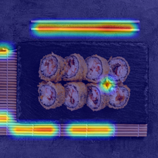
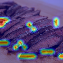
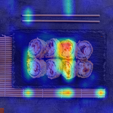
Visual Results


Cons of this method
- This methodology is not class-specific
- They end up ignoring most of the attention scores, and other layers are not even considered.
-
Gradient Attention Rollout
The Attention that flows in the transformer passes along information belonging to different classes. Gradient rollout lets us see what locations the network paid attention to, but it tells us nothing about whether it ended up using those locations for the final classification.
We can multiply the attention with the gradient of the target class output, and take the average among the attention heads (while masking out negative attention) to keep only attention that contributes to the target category (or categories).
When fusing the attention heads in every layer, we could just weigh all the attentions (in the current implementation it’s the attention after the softmax, but maybe it makes sense to change that) by the target class gradient, and then take the average among the attention heads
The main code for implementing the Gradient Attention Rollout method is as follows:
1
2
3
4
5
6
7
8
9
10
11
12
13
14
15
16
17
18
19
20
21
22
23

with torch.no_grad():
        for attention, grad in zip(attentions, gradients):
            if counter == 0:
                counter += 1
                continue

            weights = grad
            attention_heads_fused = (attention*weights).mean(axis=2)
            attention_heads_fused[attention_heads_fused < 0] = 0

            pdb.set_trace()
            # Drop the lowest attentions, but
            # don't drop the class token
            flat = attention_heads_fused.view(attention_heads_fused.size(0), -1)
            _, indices = flat.topk(int(flat.size(-1)*discard_ratio), -1, False)
            #indices = indices[indices != 0]
            flat[0, indices] = 0

            I = torch.eye(attention_heads_fused.size(0))
            a1 = (attention_heads_fused + 1.0*I)/2
            a1 = a1 / a1.sum(dim=-1)
            #pdb.set_trace()
            result = torch.matmul(a1, result)
Visual Results

TODO
So far we have presented two simple methods for explainable ViT based on attention maps and the gradient. We have tested these methods using single images for visualization purposes from the 🐶🐱 dataset. However, we haven’t yet introduced any quantified way to measure the performance of these methodologies. As a simple TODO you will need to come up with ways to measure the performance of these two methodologies. You will need to find a ground truth and compare both methodologies.
Test also the gradCAM approach for ViT models and compare the results with the previous methods quantitatively and quantitatively.
Conclusions
In this tutorial, we have analyzed the ViT model and how it works. We have developed a simple ViT classifier for the 🐶🐱 dataset and trained the model. We have also analyzed two approaches for explaining the behavior of the ViT model. The first approach called Attention Rollout is based on the Attention Maps and a way to summarize the content of the attention maps to understand the behavior of the model. The second approach is called Gradient Attention Rollout and is based on the Gradient-based methods and a way to visualize the gradient influence over the attention maps which helps as well to understand the behavior of the model. We conclude with a simple TODO exercise that will help you understand the behavior of the ViT model and the interpretability methods.