This page contains auxiliar material for this course. It contains definitions about concepts that are supplementary and optional for the ML course. It only means for the curious reader and it does not need to be read for the course sake. It contains advanced concepts for ML like vector spaces, linear independence, basis, basis transformation and matrix decomposition.

Vector redefined

As we have seen in the previous page a vector in computer science can be considered to be simply be an ordered list of numbers or things that can be eventually modelled and represented by numbers (text, audio, images etc). For example, when studying analytics on housing market and we model our problem with two only features,
thus $\mathbf{h}_1 = [55, 500K] \in \mathbb{R}^{2}$, $\mathbf{h}_2 = [105, 900K] \in \mathbb{R}^{2}$ etc, in this case the first house size is $55$ square meters and costs $500.000$€. In this example, we model our problem with two features and we can say that our vectors live in two-dimensional space or $\mathbb{R}^{2}$, the two dimensional space of all real values.

However, there is nothing in the computer science that limits a vector to lie in just two dimensions. If we have a ordered list of n-elements (for instance features for housing) then we can talk about n-dimensional vectors or $\mathbb{R}^N$. We can even talk of spaces that look like matrices or tensors. We can also talk about spaces we certain and more peculiar characteristics. For instance the space of all complex numbers, or natural numbers. The word space invite us to consider all possible vectors that exist in each of these situations.

From the geometry perspective we usually talk about 2-dimensional or even 3-dimensional vectors that represents the coordinates that we physically live in, so we can imagine or the real possible physical space. However, in algebra we can make the abstract leap can discuss about multiple and more complex dimensions. Examples of vector spaces could be the following:

$\mathbb{M}$ the vector space of all $2 \times 2$ matrices.
$\mathbb{F}$ the vector space of real functions $f(x)$.
$\mathbb{Z}$ the vector space that consists only the zero vector.

Vector spaces

A vector space is a really important definition in Linear Algebra but sometimes hard to understand and grasp. It is somehow simple but at the same time really abstract and vague. What a beauty! To grasp the reason that we need to introduce the vector space lets for a second focus or the real physical space of three-dimensions. Vector in physical space could represent quantities with both magnitude and direction. An example of that can be force, a velocity, gravity etcetera usually depicted with arrows. Length shows magnitude and the arrowhead shows direction, forming the basis of physics for describing motion and interactions. This physical space is equipped with two simple operators addition and scaling. If you add two vectors, or if you scale any vector you end-up having another vector within this physical space.

A vector space, it is an extension of the idea of physical space, but with objects (vectors) that they do not represent directly a physical meaning (like velocity, gravity etcetera) but could simple be a collection of number (data) as we have seen before and work similar with the physical spaces. They are equipped with the same properties (addition and scaling).

The reason why we study vector spaces is because they provide a useful framework for representing and solving many problems in mathematics, physics, engineering, and computer science. For example, they are used in linear algebra to study linear equations and matrices, in computer graphics to represent shapes and animations, and in machine learning to represent data.

As simple metaphors think about the LEGO blocks that could represent different vectors. The vector space is the entire collection of possible structures you can build using a set of initial LEGO blocks given to you in the box. Where where adding two structures gives another valid structure, and making a structure bigger or smaller also results in a valid structure. Another example to grasp what is going on here is with the computer graphics: A color in a game (like RGB values) can be represented by a vector, and the space of all possible colors is a vector space.

We will start with a simple example. Let’s say that we got two vectors $\mathbf{v}_1 = [1, 1] \in \mathbb{R}^{2}$ and $\mathbf{v}_2 = [1, 2] \in \mathbb{R}^{2}$. These vectors are a placeholder for two different features or we can call them dimensions, thus we say that these features belong to the $ \in \mathbb{R}^{2}$ space. That means that these features lives in the space where all two-dimensional vectors that take real values live. That space can be easily represented by the cartesian space as such:

Sublime's custom image

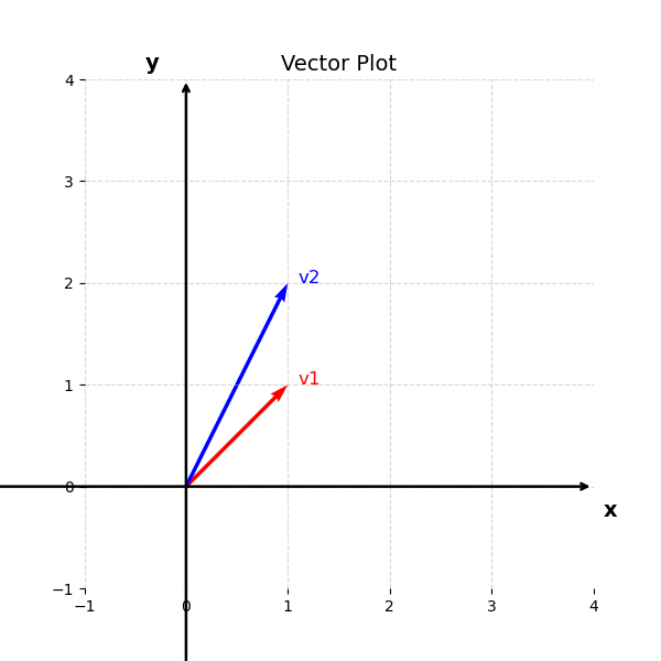
Here we can see just two vectors in two dimesions, but in the vector space of two-dimensional real vectors you can imagine all the possible vectors in the cartesian space.

The same goes with the vectors belongs to three-dimensional space like $\mathbf{v}_1 = [1, 1, 0] \in \mathbb{R}^{2}$ and $\mathbf{v}_2 = [1, 2, 1]$. In this case, we will need to visualize the vectors in three-dimensions

example with three dimensional vectors

A vector space is a collection of things called vectors, where you can:

Add any two vectors and get another vector in the space.

Multiply any vector by a number (scalar) and still get another vector in the space.

Definition:

A vector space consists of a set $V$ (elements of $V$ are called vectors), a field $F$ (elements of $F$ are called scalars), and two operations

An operation called vector addition that takes two vectors $v, w \in V$, and produces a third vector, written $v + w \in V$.
An operation called scalar multiplication that takes a scalar $c \in F$ and a vector $v \in V$ , and produces a new vector, written $cv \in V$. which satisfy the following conditions (called axioms).

Associativity of vector addition: $(u + v) + w = u + (v + w)$ for all $u, v, w \in V$.
Existence of a zero vector: There is a vector in $V$ , written $0$ and called the zero vector, which has the property that $u + 0 = u$ for all $u \in V$
Existence of negatives: For every u \in V , there is a vector in $V$, written $−u$ and called the negative of u, which has the property that $u + $(−u) = 0$.
Associativity of multiplication: $(ab)u = a(bu)$ for any $a, b \in F$ and u \in V .
Distributivity: $(a + b)u = au + bu$ and $a(u + v) = au + av$ for all $a, b \in F$ and $u, v \in V$.
Unitarity: $1u = u for all u \in V$.

Vector sub-spaces

I think an easy way to understand the sub-spaces is by providing simple examples. Lets think at fist the $\mathbf{R}^3$ vector space. Let us also imagine a plane that passes through origin $(0, 0, 0)$. That plane is a vector space by itself. If we add two vectors in the plane or scale any vector we will end-up with a vector that still passes through origin and that lives in the plane. Even though this plane looks like a 2D space, from the initial three-dimensional perspective this plane lives in three-dimensions. We can say that this plane that passes though origin is a subspace of the full $\mathbf{R}^3$ vector space.

Definition of a sub-space

A subspace of a vector space is a set of vectors included vector $\mathbf{0}$ that satisfies two requirements. If $\mathbf{0}$ and $\mathbf{w}$ are two vectors that live to our subspace and $c$ a scalar then:

$\mathbf{v} + \mathbf{w}$ belongs also to the subspace and
any $c \cdot \mathbf{v}$ or $c \cdot \mathbf{w}$ also belongs to subspace.

Basis and Rank

n linear algebra, basis helps us break down complex objects into a collection of simpler ones. A basis is a set of vectors that can represent any other vector in a given vector space. By using a basis, we can simplify computations, determine the dimension of the vector space, and perform operations in a more efficient way. We can think of basis as a set of ingredients which we can use to represent and vector in a given vector space. Similar to the previous section, we will first informally motivate the definition of a basis, and only then formalize it.

The basis of a vector space provides an organized way to represent any vector in that space. As a simple example, let’s think about possible colors produced by a pixel on the screen you are reading this on. Every pixel consists of 3 lighting elements: red, green, and blue, and every other color can be reproduced by varying the intensities of each of these colors. Since the lighting elements are independent, we can represent an arbitrary color c as follows:

\[\mathbf{c} = \begin{pmatrix} r_i \\ g_i \\ b_i \end{pmatrix},\]

where

\[\mathbf{c} = \begin{pmatrix} r_i \\ 0 \\ 0 \end{pmatrix} + \begin{pmatrix} 0 \\ g_i \\ 0 \end{pmatrix} + \begin{pmatrix} 0 \\ 0 \\ b_i \end{pmatrix}\] \[= r_i \cdot \begin{pmatrix} 1 \\ 0 \\ 0 \end{pmatrix} + g_i \cdot \begin{pmatrix} 0 \\ 1 \\ 0 \end{pmatrix} + b_i \cdot \begin{pmatrix} 0 \\ 0 \\ 1 \end{pmatrix}\]

We can now also give unique names to the column vectors and write the previous expression as follows:

\[\mathbf{c} = r_i \cdot \mathbf{r} + g_i \cdot \mathbf{g} + b_i \cdot \mathbf{b}\]