Machine Learning definition
We will start this tutorial by introducing the concept of Machine Learning (ML). A popular definition regarding ML could be the following:
Machine learning (ML) domain concerns the designing of algorithms that automatically extracts interesting information from knowledge sources that we call data.
Machine learning (ML) is data-driven and the data is at core of machine learning. The goals is to design general purposes machine algorithms with which we can extract automatically interesting patterns from the data that are not necessarily dependent in expertise domain. For instance having a huge corpus of textual data from Wikipedia we can automatically extract information about these Wikipedia sites such as the topic of each page but also event analysis or sentiment analysis in reviews from webpages such as the IMDB or Google reviews. For instance, let’s say that we have the following review from the IMDB:
Horrible script with mediocre acting. This was so bad I could not finish it. The actresses are so bad at acting it feels like a bad comedy from minute one. The high rated reviews is obviously from friend/family and is pure BS.
In this case, we create a ML algorithm that could automatically recognize that this is a review has a negative sentiment. We call this type of ML application: sentiment analysis or sentiment recognition.
Other examples of tasks that concern ML are object recognition, recommendation systems, text generation, voice detection, image generation, stock market prediction etc. Some of the ML techniques require some expertise when collecting the data and some annotation of the data. For example when we collect object as images we can annotate the content of the images with what it can be found within these images (we can collect images that contain flowers and annotate them with the name of each flower). There are some cases, that is not possible to do that, or it is not necessary to annotate these data like when we mine text from the web.
The ML systems are based on three key ingredients which are the following: data, the task and finally the the model.
We could say that in ML we use a
modelto extract interesting patterns from ourdatato perform a specifictask.
In the following section, we will mainly analyze the first concept of ML that is the data.
From data to datasets, vectors and matrices
So far, we talked about data that are crucial concept on ML but we haven’t gave any definition on what we mean when we talk about data and as a consequence what is a dataset. There are actually multiple definitions for the word data. We will try to make sense for this word by providing several definitions for this word:
Data refers to recorded observations or measurable pieces of information, often collected from experiments, transactions, sensors, texts, or user behavior, that are used to represent phenomena, derive insights, or inform decision-making through analysis.
Data are values or observations, usually structured, often numeric, that represent attributes of entities and are used to answer questions.
Data are representations of variables measured from the real world, which can be used to model and infer patterns or causality.
Central to the concept of data is the numerical representation of information about the real world about an under study domain. That involves information that we exchange as human beings or measurements that derives from scientific experiments. In both cases, the data are structured and presented in a formatted and formal way. These observations about the study phenomenon are called observations or instances. For example, if we would like to study the market value of houses in Amsterdam, we could gather information about a number of different houses (which are our observations or instances) and composed from several bits of information like:
Neighborhood,Size,Number of rooms,ConditionYear of construction,Has a balcony,Distance from the nearest tram stop,Has a jacuzziCondition of the interior,furnitureetc.
These bits of information in the nomenclature of ML is called features.
Finally, when we talk about a dataset usually we refer to structure data that are refer to a collection ofobservations. Usually, these datasets contains multiple observations which sometimes are accompanied with annotations that are curated by experts in the domain of study (think of image-scans of a patient). We can collect first scans of several patients and then an expert can annotate whether the scans contain a specific disease or not.
Types of Data
Data exists in different flavours. First and foremost could be numerical data: imagine for example the measurements of scientific tools. Scientific instruments used to quantify physical properties. These tools range from simple rulers and graduated cylinders to more advanced devices like micrometers, pH meters, and data loggers. They could be also textual data that can be found for instance in social media in forums forums etc. Could be digitalized images and audio signals. It could be boolean values (True or False). We can actually group the data into the following categories:
- Structure data (tabular data, spreadsheet).
- Unstructured data (text, images).
- Semi-Structured Data (json files).
- Time series data (audio, stock market values).
- Categorical Data (gender, race, etcetera).
- Numerical Data
Example of data
Here we will represent a simple example of gathering data about several people: name, gender, degree, postcode, age, salary with the observation to be each different person, and we would like to create an ML algorithm that given the info for these people to estimate a prediction for their salary. We can say that our observation is the different people in the Table 1.1 while the each characteristic can be called a feature. Note this table extracted by a popular dataset that studies gender biases.
Even when we have data in tabular format, there are still choices to be
made to obtain a numerical representation. For example, in Table 1.1, the
gender column (a categorical variable) may be converted into numbers 0
representing Male and 1 representing Female. Alternatively, the gender
could be represented by numbers −1, +1, respectively (as shown in
Table 1.2). Furthermore, it is often important to use domain knowledge
when constructing the representation, such as knowing that university
degrees progress from bachelor’s to master’s to PhD or realizing that the
postcode provided is not just a string of characters but actually encodes
an area in London.
Data as vectors and matrices
We just saw that not all data are inherently numerical, and from the computer perspective, it is always necessary to transform these data into a numerical representation. Thus, when we talk about digital images we talk about pixel numerical representation. Regarding textual data, each character letter, digit, symbol is assigned a number via an encoding standard, such as ASCII or Unicode (pls check this site for further information). Another example concerns auditory data which when we digitalize it, we actually captured the the amplitude of sound waves over time.
For comprehensive purposes of the humans and computers, when we collect, store and share these data we need to make use of placeholders, entities that can store information and can be easy to represent and manipulate them from mathematical perspective. Hence, we can introduce in our terminology the concept of a vector as the main placeholder of data. Vectors are used to store information about observations in our data. In the previous example, each row of the table (each different person) is considered an observation and is represented by vectors.
Dataset as we mentioned before are usually composed with a set of multiple observations, for instance when we do have a set of images we can say that each image each a different observation or a different instance. Each instance could be eventually be represented by a corresponding vector. As we said the dataset is a collection of observations and thus a collection of vectors. We can introduce also the concept of a matrix as a set of multiple vectors grouped together.
Thus, a vector (an single observation or instance) can be represented as $\mathbf{x}$, so we can have:
\[\mathbf{x}_1 = \{1, 1, 3, 41.507, 41, 9.9 \}\]and
\[\mathbf{x}_2 = \{2, 1, 1, 51.5074, 19, 1.7 \}\]while the whole dataset can be represented by the following matrix:
\[\mathbf{X} = \begin{pmatrix} 1 & 1 & 3 & 51.507 & 41 & 9.9 \\ 2 & 1 & 1 & 51.5074 & 19 & 1.7 \\ 3 & 1 & 3 & 51.607 & 27 & 7.5 \\ 4 & 2 & 2 & 51.207 & 19 & 1.6 \\ 5 & 2 & 1 & 51.407 & 20 & 1.6 \\ \end{pmatrix}\]Intro to Linear Algebra
Vectors could be regarded as placeholders from the computer science perspective, but at the same time, they can be perceived as objects in the geometric space (or Cartesian space). Therefore, they could be manipulated by Linear Algebra or geometric tools (that you might have already encounter from high-school mathematics courses). Vectors have length, direction and they live in a multi-dimensional space. We can also call them geometric vectors.
Geometric Vectors
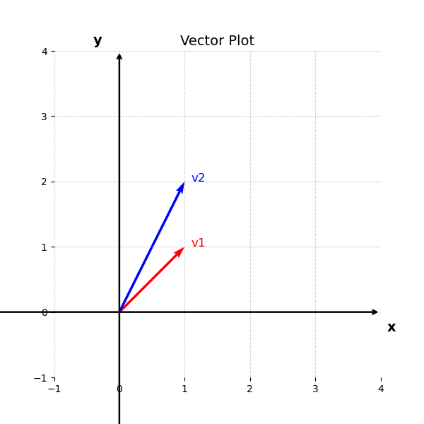
These geometric vectors are usually denoted by a small arrow above the letter, e.g. $\vec{v_1}$ and $\vec{v_2}$. In this tutorial, we will simply denote the vectors as $\mathbf{v}_1$, $\mathbf{v}_2$ as a collection of numerical values. For example we can have that:
and
\[\mathbf{v}_2 = [1, 2]\]These are examples of two dimensional vectors that lie on the cartesian space with coordinates ${x, y}$. Each dimension (or coordinate) of this vector it is called a feature and can represent a characteristic value for our observation. For example, these two value of the vector $\mathbf{v}_1$ could be the values of an image that contains just two pixels or the score of students in two different classes. Ιn general they represent observations with two-features.
You may recall from high-school that these vectors can be visualized in the cartesian 2-dimensional space as:
Once we represent our observations in vectors and visualize them in the cartesian space we can actually perform some basic mathematical computations. One simple and straightforward example is to add these two vectors. That can be represented as
\[\mathbf{v}_1 + \mathbf{v}_2 = [2, 3]\]That is represented by the following image:
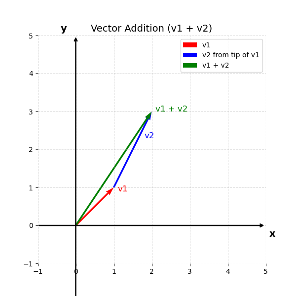
As you might recall the addition of the vectors in two-dimensions works as follows: you can start with the first vector which point to the position $\mathbf{v}_1 = [1, 1]$ and then you add one in the x-axis and 2 in the y-axis. The result of this addition is another vector that points to $\mathbf{v}_1 + \mathbf{v}_2 = [2, 3]$. This operation can be considered as a tip and tail addition. The tail here refers to the starting point of the vector, while the tip (or head) is the ending point, typically indicated by an arrowhead
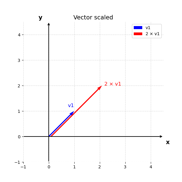
Another simply example is the multiplication of a vector with the scalar. For instance
\[\mathbf{v}_3 = 2 \cdot \mathbf{v}_1 = [2, 2]\]
Vector subtraction
What if we would like to subtract two vectors. In this case, we can simple perform vector addition, however, instead of adding the two vectors directly, we will need to add the negative of a vector, an operation that looks as follows:
\[\mathbf{v3} = \mathbf{v1} - \mathbf{v2} = \mathbf{v1} + (-\mathbf{v2})\]So in our example $\mathbf{v3} = [0, -1]$
One remark here that is good to remember is that the vectors in our example live in the two-dimensional space, and thus, it is easy to visualize. However, they could easily live in a higher dimensionality, which is also more practical, since the most interesting problems lives in a high-dimension. The only problem is that unfortunately, we cannot visualize these vectors. Thus, in this tutorial, we are usually employ two-dimensional vectors as example since it is easy also to visualize them.
Inner product
A really important concept in Linear algebra is called inner product. If we stick with the above-mentioned vectors we can calculate the following entity $\mathbf{v}_4 =\mathbf{v}_1 \cdot \mathbf{v}_2 = 1 \cdot 1 + 1 \cdot 2 = 3$. Eventually, we end up calculating a scalar value which represents the similarity of these two vectors. It shows actually if these two vectors point to the same direction they are perpendicular or point to opposite direction. Thus, the inner product:
- Is positive if the angle between vectors is less than $90^\circ$,
- Zero if the vectors are orthogonal (perpendicular),
- Negative if the angle is greater than $90^\circ$.
Another thing to keep in mind is that this product relates also with the angle between the two vectors. It ends up being as follows:
\[\mathbf{v}_1 \cdot \mathbf{v}_2 = \lVert \mathbf{v}_1 \lVert \lVert \mathbf{v}_2 \lVert \cdot cos(\theta)\]The norm of a vector
\[\lVert \mathbf{v}_1 \lVert = \sqrt{1^2 + 1^2 } = \sqrt{2} \text{, }\lVert \mathbf{v}_2 \lVert = \sqrt{1^2 + 2^2 } = \sqrt{5}\]represents the length of the vector. Here you should think of the Pythagorean theorem and how to compute the hypotenuse of a triangle side.
We can also re-write as:
\[\lVert \mathbf{v}_1^{2} \lVert = 1^2 + 1^2\]and the angle between the two vectors as:
\[cos(\theta) = \frac{\mathbf{v}_1 \cdot \mathbf{v}_2}{\lVert \mathbf{v}_1 \lVert \lVert \mathbf{v}_2 \lVert }\]Matrices
Now if we would like to create a placeholder in order to store multiple vectors together (so multiple instances), we can construct a matrix. A matrix could encapsulate the given set of observation into a rectangular entity that looks like an extended version of a vector. For instance given the observation $\mathbf{v}_1, \mathbf{v}_2$ we can group them together into a dataset or a matrix as follows:
And that can of course can be generalized with multiple vectors of n-th dimensions as follows:
\[A = \begin{bmatrix} a_{11} & a_{12} & \cdots & a_{1n} \newline a_{21} & a_{22} & \cdots & a_{2n} \newline \vdots & \vdots & \ddots & \vdots \newline a_{m1} & a_{m2} & \cdots & a_{mn} \end{bmatrix}\]with $a_{ij}\in \mathbb{R}$, where $\mathbb{R}$ is the set with all the real-values. We then can denote that a vector $\mathbf{v}_1 \in \mathbb{R}^2$ and the matrix $\mathbf{A} \in \mathbb{R}^{m \times n}$, where $\mathbb{R}^{m \times n}$ is the set of all real-valued $m \times n$ matrices.
Matrix addition
In the same spirit with the addition of a vector, we can define also the addition of two (or more) matrices. For example if we have a matrix $\mathbf{B}$ as:
\[B = \begin{bmatrix} b_{11} & b_{12} & \cdots & b_{1n} \newline b_{21} & b_{22} & \cdots & b_{2n} \newline \vdots & \vdots & \ddots & \vdots \newline b_{m1} & b_{m2} & \cdots & b_{mn} \end{bmatrix}\]Then, $\mathbf{C} = \mathbf{B} + \mathbf{A}$ can be defined as follows:
\[C = \begin{bmatrix} a_{11} + b_{11} & a_{12} + b_{12} & \cdots & a_{1n} + b_{1n} \newline a_{21} + b_{21} & a_{22} + b_{22} & \cdots & a_{2n} + b_{2n} \newline \vdots & \vdots & \ddots & \vdots \newline a_{m1} + b_{m1} & a_{m2} + b_{m2} & \cdots & a_{mn} + b_{mn} \end{bmatrix}\]It is important to note that in order to be able to add two matrices they need to have the same size otherwise it is not possible to perform the matrix addition.
Matrix multiplication
Another important operation in matrixes is the matrix multiplication. For matrices $\mathbf{A} \in \mathbb{R}^{m \times n} $, $\mathbf{B} \in \mathbb{R}^{n \times k} $, the multiplication operation can be denoted as $\mathbf{D} = \mathbf{A} \cdot \mathbf{B}$, with to be:
\[\mathbf{D} = \begin{bmatrix} d_{11} & d_{12} & \cdots & d_{1k} \newline d_{21} & d_{22} & \cdots & d_{2k} \newline \vdots & \vdots & \ddots & \vdots \newline d_{m1} & d_{m2} & \cdots & d_{mk} \end{bmatrix}\]the elements $ d_{ij} $ of the product
\[\mathbf{D} = \mathbf{A}\cdot \mathbf{B} \in \mathbb{R}^{m \times k}\]are computed as:
\[d_{ij} = \sum_{l=1}^{n} a_{il} b_{lj}, \quad i = 1, \ldots, m, \quad j = 1, \ldots, k\]Hence, in the case of matrix multiplication it is important to note that the number of columns of the first matrix should be the same for the number of rows of the second matrix in order the multiplication to be a valid operation.
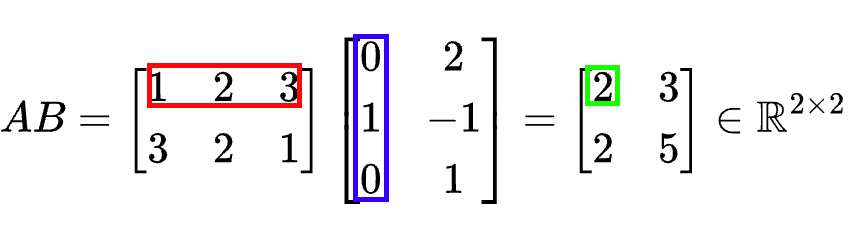
That means that in order to calculate $d_{ij}$ element we need to multiple the elements of the i-th row of $\mathbf{A}$ with the j-th column of $\mathbf{B}$ and sum them up, so to calculate the inner product of these two. Of course, a row in matrix can be considered as a vector and thus, we can just use the inner product that we can discuss earlier.
The matrices can only be multiplied if their neighboring dimensions match. For instance, an $n \times k$-matrix $\mathbf{A}$can be multiplied with a $k \times m$-matrix $\mathbf{B}$, but only from the left side:
The product $BA$ is not defined if $m \ne n$ since the neighboring dimensions do not match.
Example of matrix multiplications
An example to help you grasp the detail inner working of the matrix multiplication is placed below. By having two matrices $\mathbf{A}$ and $\mathbf{B}$:
\[\mathbf{A} = \begin{bmatrix} 1 & 2 & 3 \newline 3 & 2 & 1 \end{bmatrix} \in \mathbb{R}^{2 \times 3}\] \[\mathbf{B} = \begin{bmatrix} 0 & 2 \newline 1 & -1 \newline 0 & 1 \end{bmatrix} \in \mathbb{R}^{3 \times 2}\]we can obtain the results of multiplying $\mathbf{A}$ with $\mathbf{B}$
and the results multiplying $\mathbf{B}$ and $\mathbf{A}$:
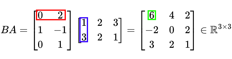
From this example, we can already see that matrix multiplication is not commutative, i.e., $\mathbf{A}\mathbf{B} \neq \mathbf{B}\mathbf{A}$;
Identity matrix
A very interesting and useful type of matrix is called identity matrix. The properties of this matrix is that every item of the matrix is zero except the diagonal of the matrix where the value is equal to one. An example of this matrix can be found as follows:
\[\mathbf{I}_n := \begin{bmatrix} 1 & 0 & \cdots & 0 & 0 \newline 0 & 1 & \cdots & 0 & 0 \newline \vdots & \vdots & \ddots & \vdots & \vdots \newline 0 & 0 & \cdots & 1 & 0 \newline 0 & 0 & \cdots & 0 & 1 \end{bmatrix} \in \mathbb{R}^{n \times n}\]You should note that the identity matrix is always squared meaning that it has the same number of rows and columns which is represented by the number $n$.
Matrix properties
There are a lot of properties that stem from the previous mentioned operations (addition and multiplication)
- Associativity: $ \forall \mathbf{A} \in \mathbb{R}^{m \times n}, \mathbf{B} \in \mathbb{R}^{n \times p}, C \in \mathbb{R}^{p \times q} : (\mathbf{A}\mathbf{B})\mathbf{C} = \mathbf{A}(\mathbf{BC}) \tag{2.18}$
-
Distributivity: $ \forall \mathbf{A}, \mathbf{B} \in \mathbb{R}^{m \times n}, \mathbf{C}, \mathbf{D} \in \mathbb{R}^{n \times p} : (\mathbf{A} + \mathbf{B})\mathbf{C} = \mathbf{A}\mathbf{C} + \mathbf{B}\mathbf{C} \tag{2.19a}$, $\mathbf{A}(\mathbf{C} + \mathbf{D}) = \mathbf{AC} + \mathbf{AD}$
-
Multiplication with the identity matrix: $ \forall \mathbf{A} \in \mathbb{R}^{m \times n}$: $\mathbf{I}_m \cdot \mathbf{A} = \mathbf{A} \cdot \mathbf{I}_n = \mathbf{A}$
- Inverse and Transpose
Consider a square matrix $\mathbf{A} \in \mathbb{R}^{n \times n}$. Let matrix $\mathbf{B} \in \mathbb{R}^{n \times n}$ have the property that $\mathbf{AB} = \mathbf{I}_n = \mathbf{BA}$. $\mathbf{B}$ is called the inverse of $A$ and denoted by $\mathbf{A}^{-1}$.
Unfortunately, not every matrix $A$ possesses an inverse $\mathbf{A}^{-1}$. If this inverse does exist, $\mathbf{A}$ is called regular-invertible-nonsingular, otherwise singular-noninvertible. When the matrix inverse exists, it is unique. There are ways to determine whether a matrix is invertible but this is out of the scope of the mathematics intro.
Inverse of a matrix
Let us assume two matrices $\mathbf{A} \in \mathbb{R}^{n \times n}$ and $\mathbf{B} \in \mathbb{R}^{n \times n}$. If the following property is true: $\mathbf{A} \cdot \mathbf{B} = \mathbf{I}_n$, then we can say that $\mathbf{B}$ is the inverse of matrix $\mathbf{A}$.
For instance if we have the following matrices:
\[\mathbf{A} = \begin{bmatrix} 1 & 2 & 1 \newline 4 & 4 & 5 \newline 6 & 7 & 7 \end{bmatrix} \in \mathbb{R}^{3 \times 3}\]and
\[\mathbf{B} = \begin{bmatrix} -7 & -7 & 6 \newline 2 & 1 & -1 \newline 4 & 5 & -4 \end{bmatrix} \in \mathbb{R}^{3 \times 3}\]Then the product $\mathbf{A} \cdot \mathbf{B} = \mathbf{I}_3$
Transpose of a matrix
Another definition that we will encounter in this course is the transpose matrix. So if we have two matrices again $\mathbf{A} \in \mathbb{R}^{n \times m}$ and $\mathbf{B} \in \mathbb{R}^{m \times n}$, then we call matrix $\mathbf{B}$ as the transpose matrix $\mathbf{A}$ if the transpose matrix of $\mathbf{B}$ denoted as $\mathbf{B}^T$ is equal with matrix $\mathbf{A}$, $\mathbf{A} = \mathbf{B}^T$. Thus, if we calculate the transpose of $\mathbf{A}^T$ from the previous example then, we can calculate the following:
\[\mathbf{A}^T = \begin{bmatrix} 1 & 4 & 6 \newline 2 & 4 & 7 \newline 1 & 5 & 7 \end{bmatrix} \in \mathbb{R}^{3 \times 3}\]We can say that the rows of the initial becoming the columns of the transpose matrix. Now several interesting properties for inverse and transpose matrices arise:
\[\mathbf{A} \cdot \mathbf{A}^{-1} = \mathbf{I} = \mathbf{A}^{-1} \cdot \mathbf{A}\] \[\mathbf{(AB)}^{-1} = \mathbf{A}^{-1} \cdot \mathbf{B}^{-1}\] \[(\mathbf{A+B})^{-1} \neq \mathbf{A}^{-1} + \mathbf{B}^{-1}\] \[(\mathbf{A}^T)^{T} = \mathbf{A}\] \[\mathbf{(AB)}^{T} = \mathbf{B}^{T} \cdot \mathbf{A}^{T}\] \[(\mathbf{A+B})^{T} = \mathbf{A}^{T} + \mathbf{B}^{T}\]Linear systems
A simply way to understand the usefulness of matrices and vectors stems from the linear system world (as you might recall from the high-school). We can define as a linear system a collection of linear equations that involve the same set of variables.
To better grasp this let us for a second try to solve the following problem movie-recommendation. We do have the following scenario:
A movie platform wants to understand a user’s taste based on three factors:
- $w_1$ $\rightarrow$ the intensity of action characteristics.
- $w_2$ $\rightarrow$ the intensity of romantic-comedy characteristics.
- $w_3$ $\rightarrow$ the intensity of horror-style characteristics.
The system observes how the user rated three different movies (on a 1–10 scale). Each movie has known feature intensities (e.g., how much action, romance, and horror it has). The rating for the first movie is 7, for the second 9 and the third 5. The platform tried to understand the interest of the user. That problem can be represented by the following linear system of equations:
Now, if we define as:
\[\mathbf{X} = \begin{bmatrix} 2 & 3 & 1 \newline 3 & 2 & 2 \newline 1 & 4 & 3 \end{bmatrix} \in \mathbb{R}^{3 \times 3}\]And then we can define
\[\mathbf{w} = [w_1, w_2, w_3] \in \mathbb{R}^{3 \times 1}\]and
\[\mathbf{y} = [y_1, y_2, y_3] = [7, 9, 5] \in \mathbb{R}^{3 \times 1}\]then we can simply write $\mathbf{X} \cdot \mathbf{w} = \mathbf{y}$ or simply $\mathbf{y} = \mathbf{X} \cdot \mathbf{w}$ which stems from the properties of matrix multiplication. So in essence we can see the matrix multiplication as a simple way to represent linear equations of multiple variables $\mathbf{w} = [w_1, w_2, w_3]$.
We can use also the following representation:
\[\begin{pmatrix} 2 & 3 & 1 \newline 3 & 2 & 2 \newline 1 & 4 & 3 \end{pmatrix} \begin{pmatrix} w_1 \newline w_2 \newline w_3 \end{pmatrix} = \begin{pmatrix} 7 \newline 9 \newline 5 \end{pmatrix}\]Now, we want to solve this system to figure out how much this user likes action, romantic and horror movies in general.
It can be proven that by using also the matrix properties for inverse matrices we can solve this linear equation problem and calculate the variables $\mathbf{w}$ as follows:
\[\mathbf{w} = \mathbf{X}^{-1} \cdot \mathbf{y}\]The final results can be found to be the following:
\[\mathbf{w} = [w_1, w_2, w_3] = \begin{bmatrix} 1.8 \\[4pt] -4.87 \\[4pt] 2 \end{bmatrix}.\]Thus, we have transformed the linear equation problem to matrix inverse and matrix computation in order to find a solution. That is something that we need to keep in mind that is omnipotent in machine learning. We are usually trying to solve a similar equation given a matrix $\mathbf{X}$ that represents our data.
Matrix transformations
Another way to regard matrices in general are as linear functions. That means if we have an input vector $\mathbf{w}$ and we multiply it with a matrix $\mathbf{X}$ we end up transforming the initial vector to a new one. Thus, matrix here plays the role of linear function or more usually called linear transformation.
The idea here is that when we perform $\mathbf{X} \cdot \mathbf{w} = \mathbf{y}$ then we can see $\mathbf{w}$ as our input and $\mathbf{y}$ out output. Matrix $\mathbf{X} $ can be considered as a function transformation f that maps input vector to the output vector. We can say that $\mathbf{X} \in \mathbb{R}^{n \times n}$ what it does is to receive an matrix $\mathbf{w} \in \mathbb{R}^{n}$ and it spits out a vector $\mathbf{y} \in \mathbb{R}^{n}$. Depending of the dimensionality of the matrix $\mathbf{X}$ this transformation could keep the same dimensionality or change the dimensionality of the output vector.
A nice outcome of the above is that we can even visualize the affect of matrix transformation. Therefore, in this part of the tutorial we will put forwards some classic examples of matrix transformation that can help grasp some intuitions on what it means to multiple a vector with the matrix. Let us say that we do have a vector:
\[\mathbf{v}_2 = [1, 2]\]and the matrix:
\[\mathbf{I}_2 = \begin{pmatrix} 1 & 0 \newline 0 & 1 \end{pmatrix}\]If we multiple $\mathbf{v}_2 \cdot \mathbf{I}_2$ its easy to figure out that we end up having as a result the same vector $[1, 2]$.
If we instead multiply $\mathbf{v}_2$ with matrix $\mathbf{A}$:
\[\mathbf{A} = \begin{pmatrix} a & 0 \newline 0 & b \end{pmatrix}\]That will return a slightly different vector which is $[a, 2\cdot b]$, so this diagonal-matrix $\mathbf{A}$ (only the diagonal values are non-zero) scales the values of the vector. Another example matrix is:
\[\mathbf{A} = \begin{pmatrix} 1 & 0 \newline 0 & -1 \end{pmatrix}\]which actually flips the y-axis of the vector in the negative direction. As a final example, we have matrix $\mathbf{C}$:
\[\mathbf{C} = \begin{pmatrix} 0 & -1 \newline 1 & 0 \end{pmatrix}\]which actually rotates a vector $90^\circ$. This can be validated by the following:
\[\mathbf{v}_2 \cdot \mathbf{C} = [1, 2] \cdot \begin{pmatrix} 0 & -1 \newline 1 & 0 \end{pmatrix} = [-2, 1]\]To better understand what happened, we can visualize vector $\mathbf{v}_2$ and the result of transformation:
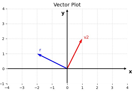
So there is always some geometric interpretation of the result of the matrix-vector multiplication. This can be extended for the matrix-to-matrix multiplication.
Distance between vectors
Nice! As a quick recap, so far we have seen that we can express instances that represent observations from real-world (or experiments) as vectors. Each different value of the vector that is called a feature represents a different measurement for the instance (or otherwise called dimension). We actually discuss also some basic tool in Linear algebra that helps us manipulate these vectors.
It is really useful also to introduce a notion of distance with which we can measure the closeness of vectors. In this way, we can compare different instances and judge which one are close or far to each other. We saw that these vectors can represent images or text. If for example they represent images, and we want to build an web-image-recommendation system like Google Lens we will need a distance measurement to figure out which images are closer to the query image at time.
Having represent the query image as a vector and all the images as vectors we can easily also use this distance metric to compute the closeness of the query image with all the images in our dataset.
If we have two vectors $\mathbf{x} = (x_1, x_2, \cdots, x_n )$ and $\mathbf{y} = (y_1, y_2, \cdots, y_n)$ a very popular distance is the Euclidean distance which can be defined as:
\[\text{Dis}_2(\mathbf{x}, \mathbf{y}) = \sqrt{(x_1 - y_1)^2 + (x_2 - y_2)^2 + \cdots + (x_n - y_n)^2}\] \[= \sqrt{\sum_{j=1}^{d} (x_j - y_j)^2}\] \[= \sqrt{(\mathbf{x} - \mathbf{y})^\top (\mathbf{x} - \mathbf{y})}\]Another way is to use 1-norm distance which is the following:
\[\text{Dis}_1(\mathbf{x}, \mathbf{y}) = {\sum_{j=1}^{d} ||(x_j - y_j)||}\]The generalized version of the previous distances is called Minkowski distance and it is as follows:
The main take-home message in this sub-section is that we can make use one of the previous tools as a means to gauge the closeness of two vectors. By employing such a tool we can create powerful Machine Learning tools.
Vector projection (and rejection)
In Linear Algebra we call orthogonal projection of vector $\vec{a}$ to $\vec{b}$ (from the below figure) and the legs (or catheti) to hypotenuse that is $\vec{a}$ are $\vec{a_1}$ and $\vec{a_2}$. The leg that is parallel with the vector $\vec{b}$ is the actually projection that we are looking for $\vec{r1}$.
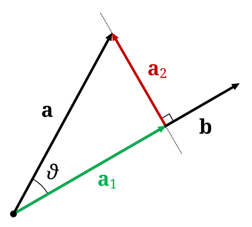
This projection is calculated as:
\[p_\vec{b} \vec{a} = \frac{a \cdot b}{||a||||b||} b\]while just the length of the projection is
\[d = \frac{a \cdot b}{||a||||b||}\]Vectors as datasets
Now lets say that we are conducting an experiment and we gather observations (instances) that lives in two dimensions. We can plot the results of these observations in a cartesian two-dimensional plot as follows:
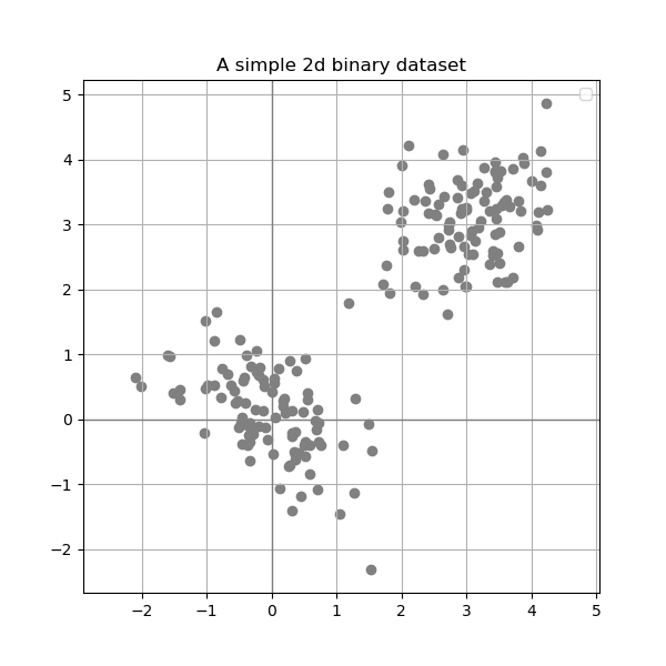
If our observations regards students and the features are student grades on Mathematics and Physics in high school.
Given that we know that these observations belongs to two distinct classes (lets say bachelor and master students) and these classes can be represented as follows:
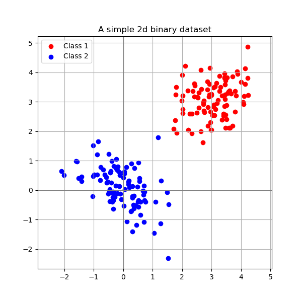
Now, two popular techniques in Machine learning are clustering and classification. In the first category, we are trying to assign for each instance a belonging class. In this case, we only have information about the instances. In the latter, while we would like to do the same thing, however, in this case, we do already have information about the class belonging of each sample. We thus want to use also this information to learn a way to separate between the known classes given the annotated information.
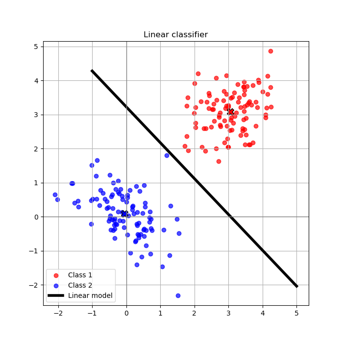
Thus, knowing the class belonging, we are looking for a line that separates the two classes. That can be seen in the following image;
Of course the most of the problems lies in a higher dimensionality that the previous problem. We can consider the case of three dimensions which can be also visualized as:
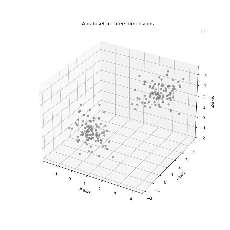
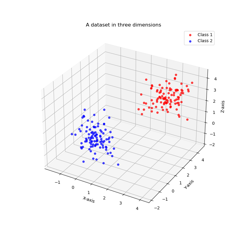
But we can also speak for higher than three dimensions. This is the case of the most interesting problems, however, it is impossible to visualize the values of these problems in a similar way. In this course, to help you with the understanding of key concepts we will make use of example datasets with two or three dimensions to explain nuances and then, we will assume that the same concepts can be generalized in higher dimensions.
Linear models in Machine learning
But ok seriously, why do we even mentioned all these above calculations and linear algebra tools for vectors and matrices. We are just interested in data and making machines more clever.
The reason why we mess with these placeholders and their mathematical properties is multi-facet.
- Firstly, is somehow intuitive to place numerical entities in boxes that look like
vector, matrices. - Moreover, it ends up being a convenient abstract representation of how the placeholders in computer looks like.
- We can use a lot of calculation tools that are provided by linear algebra and calculus and optimization to work with our data.
- Having placed all our data observations in placeholders (
vectors) we can now make use of computation tools to measure similarities and be able to group together things. Pythonhas a lot of nice packages that we can use to process our data. You will familiarize with them in the three assignments of this course. More info regarding the assignment you will be able to find here.
In the following paragraphs, we will introduce an example of a dataset and a model that performs the task of linear classification.
Example MNIST
Now, lets say that we would like to study images with handwritten digits and the classification of them into the correct digit. Each time that you write in a paper a numerical digit, scan the document, you would like your machine learning algorithm to recognize the digit.
For this purpose, we can employ a set of image-examples from the popular MNIST dataset (developed some decades ago) that contains 70.000 gray scale images of handwritten digits (with pixel size of $28 \times 28$) which are named (or labelled or annotated) after the digit that they represent. So there is a way to know what each image represents. That type of naming is called a label or an annotation. We can represent this label using an integer variable that takes the following values $t = {0, 1, 2, …, 9}$.
Each input image can be represented as a vector after placing each row next to each other. Eventually, instead of $28$ rows with $28$ columns we can end up having $1$ row with $784$ columns matrix. We can actually use as placeholder a vector $\mathbf{x} \in \mathbb{R}^{784}$. Finally, we can store all the vector-images in one big matrix:
\[\mathbf{X} = \begin{bmatrix} \text{---} & \mathbf{x}_1 & \text{---} \newline \text{---}& \mathbf{x}_2 & \text{---} \newline \vdots & \vdots & \vdots \newline \text{---} & \mathbf{x}_n & \text{---} \end{bmatrix} \in \mathbb{R}^{70000 \times 784}\]Where each row is represented by a vector $\mathbf{x}_i$. Out task is to extract useful information and patterns from these data. For example in digit-classification, we would like to build a ML model to predict automatically the digits in MNIST images without using the information from the naming or the labels. Once we build this system, we can apply to each image that contains handwritten digits and create our OCR software.
Now back to the MNIST dataset. We can actually place all the labels for each image in a single vector $\mathbf{t} \in {(0, 1, 2, …, 9)}^{70000}$.
Task example: linear classifier
A simple approach to create our first classifier (our machine learning model) is as follows:
- Introduce some parameters (we can call them also variables or
weights) $\mathbf{w}$. - Then, we simply :) need to tune these parameters in such a way that each time that we will have a new observation $\mathbf{x}^{\prime}$ that contains a handwritten digit (that we do not know beforehand its
label) - if we multiply this new instance (by using the
inner productdiscussed before) with parameters $\mathbf{w}$ the output should be a numerical value that will represent the digit that the input observation contains.
Now the whole point of tuning the parameters $\mathbf{w}$ is that we need to end up with $\mathbf{y}$ that should be always as close as possible to the desired digit value $\mathbf{t}$.
For instance if we do have as our new observation the following digit $\mathbf{x}’$:
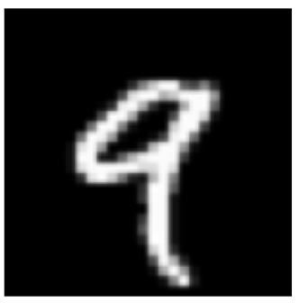
the first thing to do is that we place each row of pixels next to each other and we finally we can have a vector that looks as follows (note this is a part of the final vector and not full vector):

Then, the output of the ML model should be something like $y = \mathbf{w} \cdot \mathbf{x}’ \approx 9$ (or some other value that codifies this specific digit- that is not important for now, if you are curious make questions on it).
Note that we can have instead of a scalar a vector as an output. This vector could be $\mathbf{y} \in \mathbb{R}^{9}$ where each dimensionality represents each of the desired digits. In this case, we should replace $\mathbf{w}$ with a matrix. But for now, we will stick to the simple case of the scalar output.
Tuning phase for the parameters (training phase)
In Machine Learning we are trying to figure out a good way to tune these parameters $\mathbf{w}$ in such a way that the above classification task will be resolved. The process of tuning these parameters is called in machine learning training or learning process.
We will introduce this process with a very simplistic example that works as a basis to understand the whole concept. This should work as a mere blueprint in order to grasp the idea behind training a ML algorithm. During the lecture we will analyze several training methodologies and algorithms in more details that work in practice for multiple tasks (classification, regression, clustering etcetera).
Firstly, we will start by making a simplistic hypothesis that our data are linearly separable meaning that we could find a simple line or a surface plane in multi-dimensional space that could separate each different class for our problem.
This should be done by just performing a simple linear operation between the data in the dataset and the introduced parameters $\mathbf{w}$. This operation looks like:
\[\mathbf{y} = \mathbf{X} \cdot \mathbf{w}\]Now a very good question is the following: how can we engineer meaningful values to these parameters $\mathbf{w}$ to perform handwritten classification? The next step gives a simplistic example that could be the starting skeleton
of a ML algorithm:
- First thing first, is to access a dataset of handwriting images (MNIST) that contains some annotation or label describing whats the digit representation of its image.
- Each image $\mathbf{x}_i$ contains a label $t_i$.
- We can split this dataset into two sets: training and test set. The training set we will use it during the training phase where we will tune the parameters of the model.
- Them, the test set will be used for evaluating the quality of the tuned parameters of our new model.
Having prepared our data now we can proceed in the so-called training process, which is usually as follows (another reminder that his is a very simplistic example):
- We start by tuning these parameters $\mathbf{w}$ randomly. Having done that, now, we can calculate the output $\mathbf{y}$ using the previous linear equation $\mathbf{y} = \mathbf{X} \cdot \mathbf{w}$.
- However, given that we initialize the parameters $\mathbf{w}$ randomly there is not any quarantee that the values $\mathbf{y}$ could codify any meaningful information related to MNIST dataset.
- Meanwhile, we already know how this output should be (the stored label information $\mathbf{t}$).
- It is natural to measure the distance between the predictions $\mathbf{y}$ and the annotations $\mathbf{t}$ and then update the values of $\mathbf{w}$ in a way that this distance (think about the distance metrics we talked before) between the two vectors is minimized.
- In this way, we can measure the total error between the model output and the real labels. This is called alternatively
loss functionorerror function. - Then we can use this loss output as a compass to modify our parameters $\mathbf{w}$ and direct them towards minimizing this entity. After all, we want to minimize this distance between correct label and the predicted values.
- Throughout this course, we will analyze several key ways of tuning our parameters given this error calculation.
Hooray, we have just given a very simple explanation of how classification and supervised learning works in Machine Learning.
Of course, the whole training problem is a lot more involved that our previous description. One of the initial hypothesis that we made is that our data are linearly separable and we can use a surface to separate its classes. However, this is not the case in the most of the data. This example meant to be a gentle introduction on how the linear classification looks like.
Hence, the learning objective for this course is to make clear on how ML algorithms works and how the above-mentioned steps works in practice in more details. Furthermore, there is a huge range of problems beyond classification that ML deals with like: regression, clustering, dimensionality reduction and generation of data that we will revise in this course. Finally, you should also note that the example that we have place is an example of parameter-based classification, but classification can be done also without using explicitly new parameters $\mathbf{w}$ and by only creating rules based on data (for instance in the case of decision trees).
The main key-home messages for this page is that information and human observations are represented by data can be stored in placeholders which can be manipulated by computers using Linear algebra principles. ML is using Linear Algebra tool to do its job and tune the parameters in the desired way.
Geometry of linear classifiers
Let us assume that we do have a linear separable binary dataset (class A and B) as depicted in the following figure:
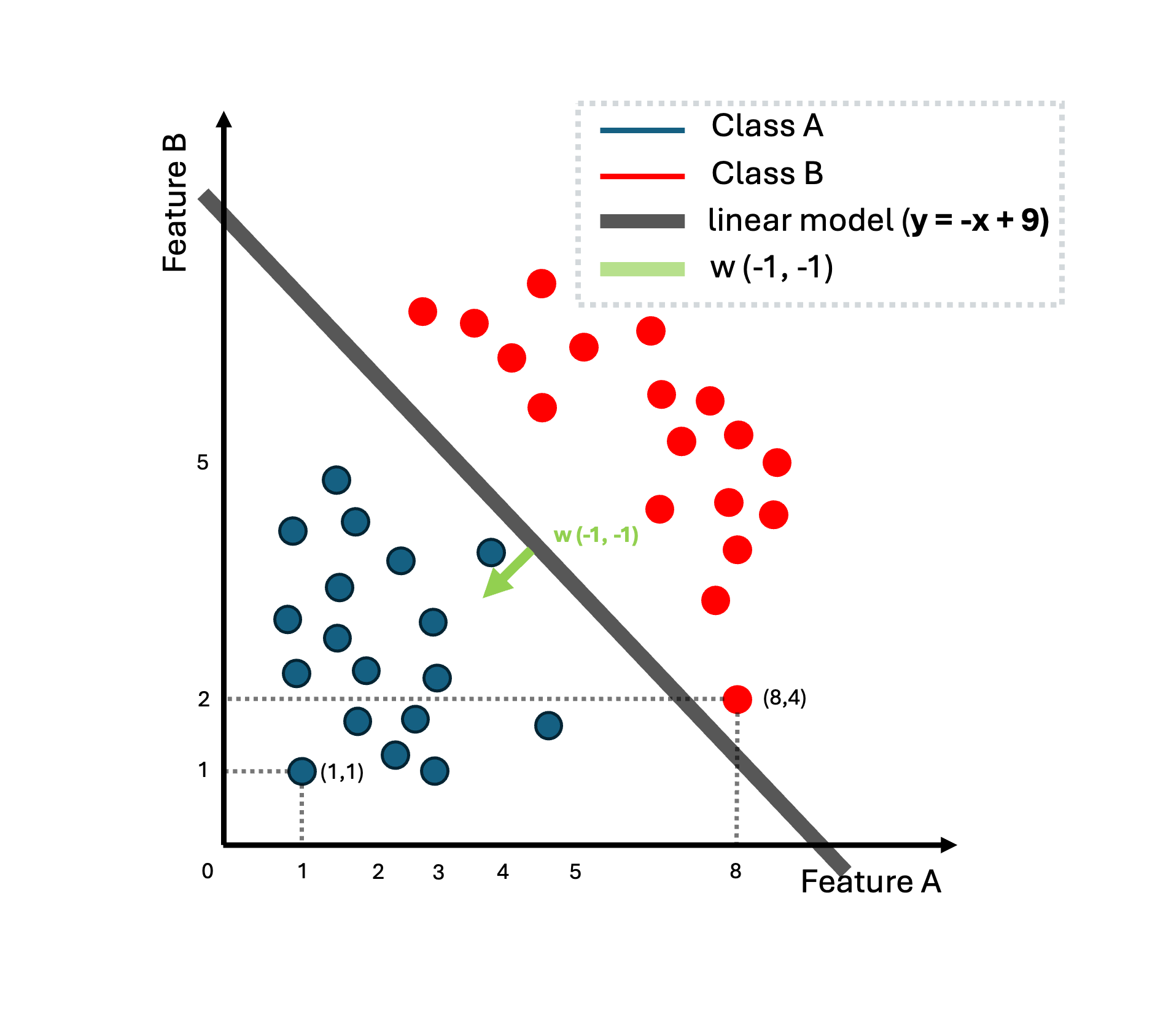
It is clear that we can find a line that separates the two classes. For instance, the following equation
\[y = -x1 -x2 + 9 = 0\]could separate the two classes. We can alternative write :
\[y = \mathbf{w}^{T}\mathbf{x} + w_0\]We thus introduce some parameters $\mathbf{w}, w_0$ (parameter $w_0$ is also called sometimes $b$) and the idea is to tune these parameters to find a decision line that separates the two classes. Our data lives in two dimensions $\mathbf{x} \in \mathbb{R}^{2}$. Thus, the linear function maps input $y: \mathbb{R}^2 \to \mathbb{R}$ to a value and when $y = 0$ we have the decision boundary for the two classes and when $y>0$ we do have a region for the class B and when $y<0$ for class A. Βy tuning these parameters $\mathbf{w}, w_0$, for instance $\mathbf{w}^{T} = [-1, -1]$ and $w_0 = 9$, we found a way to separate the two given classes.
In principle, the idea behind linear classification is to find the ideal parameters that can separate the two classes. In this chapter, we will discuss the geometry behind linear classification and several strategies to optimize and find good parameters.
Simple geometry exercise using linear algebra
Imagine that we do have two vectors $\mathbf{x}_A, \mathbf{x}_B$ that live in the decision boundary line . For the points that live in the decision line we know that this is true $y = 0$. Thus, by definition, $y_A = y_B = 0$ or we can develop further,
\[\mathbf{w}^T \mathbf{x}_A + b = \mathbf{w}^T \mathbf{x}_B + b = 0\]and by performing simple vector calculations we have:
\[\mathbf{w}^T ( \mathbf{x}_A - \mathbf{x}_B) = 0\]We already have mentioned that when the dot product of two vectors is zero then, the two vectors are orthogonal. Thus, $\mathbf{w}$ and $\mathbf{x}_A - \mathbf{x}_B$ are orthogonal to each other. Now, what we need to take into account also is that vector $\mathbf{x}_A - \mathbf{x}_B$ is always parallel to the decision boundary.
Eventually, the vector $\mathbf{w}$ and $\mathbf{x}_A - \mathbf{x}_B$ are orthogonal to each other (or perpendicular). It is also well-known in linear
algebra that the subtraction of two vector that lie in the same line, the result of subtraction will always point parallel to the line itself. Thus the final conclusion, that the vector of weights
always point perpendicular to the decision boundary. This gives us the slope of the line.
It is also easy to extract that the parameter $w_0$ or sometimes $b$ is the offset of the line and reveals how far the line is from the original $(0, 0)$.
We know also that
\[y= \mathbf{w}^{T}\mathbf{x} =0\]is a vector that point to the decision line, but it also passes through the origin.
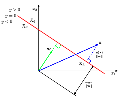
Officially, to compute the distance between the boundary and the origin we will need to pick this vector that lies in in boundary and calculate the projection of this vector to the intercept $\mathbf{w}$. That is actually the case due to the Euclidean distance. We saw before that the projection of a vector over another is computed as:
\[d = \frac{\mathbf{w}^{T}\mathbf{x}}{||\mathbf{w}||}\]since $\mathbf{w}^{T}\mathbf{x} + w_0 = 0$, we can write:
\[d = \frac{-w_0}{||\mathbf{w}||}\]Finally, we can conclude that the general distance a vector in space fom the decision boundary can be computed as:
\[d = \frac{y(\mathbf{x})}{||\mathbf{w}||}\]The proof for that should be considered as a given and it is trivial to be made. If you feel curious on it please ask us during the lecture or tutorials of the course. The main principle behind Support Vector Machines (SVM) is that we would like to find parameters $\mathbf{w}, w_0$ in such a way that the distance of the closest vectors to the decision boundary will be maximized.
The ingredients of ML
To conclude and come back to our EoML course, during the lectures, we defined as key ingredients of ML the following concepts: data (instances, features), the task, and the model.
In the previous example, we defined that a single image $\mathbf{x}$ acts as the instance or observation and its pixel-value as the feature. Our dataset is a set of images that could include annotation in the case of supervised learning and linear classification like the case of the MNIST datasets. However, we might still have a set of images without annotation and can still employ algorithms that find interesting patterns in data (clustering, image compression or image generation using GANs or stable diffusion models).
In this tutorial, we mainly focused on the linear classification task. The model is actually the parameters $\mathbf{w}$ that we introduced during the example and tuned during the training process. Thus, for each different task we have different type of a model and different type of introduced parameters $\mathbf{w}$ that needs to be learned. Think of different the different recipes for supervised or unsupervised learning and the introduced parameters.
##
Here our quick introductory story in ML ends. I am sure that this content can be a bit hard to parse for some, however, this page means to be a supplementary material for those are curious to learn more on linear algebra and mathematics for Machine Learning.