Matrix decompositions

So what is matrix decomposition? And why do we need it? This is what we will try to answer in this tutorial.

In general we have seen in previous tutorials how mappings and transformations of vectors can be conveniently seen as linear transformation and described asmatrices. We saw how data can be represented by matrices where the rows of the matrix for example represent different people or as they called instances and the columns describe different features of the people, such as: weight, height, and other information about the individuals. That row and column order does not play a really important role and we can have each instance to be a column vector so a column of the matrix. That is simply a transpose of the initial matrix.

In ML the most interesting and challenging problems are coupled with data that live in high-dimensionalities such as images, videos, brain scans etcetera. This high-dimensionality comes with multiple problems such as it makes the ML algorithm hard to parse data to interpret them while it is merely impossible to visualize them and really expensive to store the data in servers. At the same time, there are properties of these high-dimensional data that we can take advantage of. For instance, many dimensions are redundant since they could simply represented a linear combination of other dimensions. Dimensionality reduction exploits structure and correlation and allows us to work with a more compact representation of the data, ideally without losing information. We can think of dimensionality reduction as a compression technique, similar to jpeg or mp3, which are compression algorithms for images and music.

In this part of the tutorial, we will see the real merit and the reasons why we would like to perform matrix decomposition in Machine Learning. A direct answer to that is that matrix decomposition paves the way for dimensionality reduction and the discovery of embeddings that can meaningfully characterize the initial feature space of our data in hand. In this page, we will present three different aspects of these matrices:

• how to summarize matrices,
• how matrices can be decomposed,
• and how these decompositions can be used for matrix approximations.

Matrix decompositions usually decompose an original matrix into a product of simpler matrices, which have some specific features. In this theory page, we cover two important decompositions: Eigenvalue decomposition (Diagonalization) and Singular value Decomposition (SVD). Finally we show that one of the most important algorithms in Machine Learning called Principal Component Analysis (PCA) is based on matrix decomposition and SVD.

Summarizing matrices

We will start our journey by considering methods that allow us to describe matrices with just a few numbers that characterize the overall properties of matrices. These methods are the determinants, traces and eigenvalues.

Determinant of a matrix

Let’s assume a square matrix $\boldsymbol{A} \in \mathbb{R}^{n \times n}$. W use the following notation for the determinant of this matrix:

\[\det(A) = \begin{vmatrix} a_{11} & a_{12} & \ldots & a_{1n} \\ a_{21} & a_{22} & \ldots & a_{2n} \\ \vdots & \vdots & \ddots & \vdots \\ a_{n1} & a_{n2} & \ldots & a_{nn} \end{vmatrix}\]

Determinant is a function that maps a matrix into a scalar value $\det(A) \in \mathbb{R}$. The determinant is the entity that we use to check whether a matrix is invertible. It holds that if a matrix $\boldsymbol{A}$ is invertible then $\det(A) \neq 0$. That means that we cannot compute $\boldsymbol{A}^{-1}$ In case, that $\det(A) = 0$ then the matrix is not invertible and it is called a singular matrix.

The notion of a determinant is natural when we consider it as a mapping from a set of $n$ vectors spanning an object in $\mathbb{R}^n$. It turns out that the determinant $\det(A)$ is the signed volume of an $n$-dimensional parallelepiped formed by columns of the matrix $\boldsymbol{A}$.

To better grasp this, we can start with the following example: Let’s say that we got two vector $\mathbf{g} = [g, 0]^T$ and $\mathbf{b} = [0, b]^T$ in standard basis ${\mathbf{e}_1 = [1, 0]^T \mathbf{e}_2 = [0, 1]^T }$:

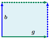
and we can place them in the following matrix:

\[\det(A) = \begin{vmatrix} g & 0 \\ 0 & b \end{vmatrix}\]

In this case, we define as determinant to be:

\[det(A) = g\cdot b + 0 = g\cdot b\]

which is the area of the parallelogram defined by the two vectors. The same happens in the below image, where we can compute the area in the $\mathbb{R}^{3}$ space using the determinant of the matrix that contains the vectors:

\[\boldsymbol{A} = \begin{vmatrix} \mathbf{g} & \mathbf{b} & \mathbf{r} \end{vmatrix}\]

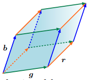
If for example we do have:

\[r = \begin{bmatrix} 2 \\ 0 \\ -8 \end{bmatrix}, \quad g = \begin{bmatrix} 6 \\ 1 \\ 0 \end{bmatrix}, \quad b = \begin{bmatrix} 1 \\ 4 \\ -1 \end{bmatrix}\]

Then, the volume of these three vectors can be found in we compute $det(A)$:

\[\det(A) = \begin{vmatrix} 2 & 6 & 1 \\ 0 & 1 & 4 \\ -8 & 0 & -1 \end{vmatrix} = 186\]

One prerequisite is that the vectors are linearly independent otherwise we cannot compute the volume. Let us imagine that the vectors $\mathbf{b}$ and $\mathbf{g}$ are dependant, that means that they are parallel. Thus the area that they define is equal to zero. That observation is really important! If a matrix contains columns that are linearly dependant then, the determinant is equal to zero and thus we can say that this matrix is a singular matrix.

The important messages in this section:

• If the determinant of a matrix is not zero, then, it represents the volume that the n column vectors define is $\mathbb{R}^{n}$ space.
• We can compute the determinant only for square matrices.
• If the matrix contains columns that are linearly dependant then we have a singular matrix.

Trace of a matrix

The second important way to summarize a matrix is by using a function called trace. This function takes as input $\boldsymbol{A} \in \mathbb{R}^{n \times n}$ and maps it into real-world values $\mathbb{R}$ in the following way:

\[tr(\boldsymbol{A}) = \sum_{i=1}^n a_{ii}\]

where $a_{ii}$ are the diagonal elements of the squared matrix.

The trace satisfies the following properties:

• $tr(\boldsymbol{A} + \boldsymbol{B}) = tr(\boldsymbol{A}) + tr(\boldsymbol{B})$ for $\boldsymbol{A}, \boldsymbol{B} \in \mathbb{R}^{n \times n}$
• $tr(\alpha \cdot \boldsymbol{A}) = \alpha \cdot tr(\boldsymbol{A})$, $\alpha \in \mathbb{R}$ for $\boldsymbol{A} \in \mathbb{R}^{n \times n}$
• $tr(\boldsymbol{I}_n) = n$
• $tr(\boldsymbol{AB}) = tr(\boldsymbol{BA})$ for $\boldsymbol{A} \in \mathbb{R}^{n \times k}$, $\boldsymbol{B} \in \mathbb{R}^{k \times n}$

It can be shown that only one function satisfies these four properties together – the trace (Gohberg et al., 2012).

The properties of the trace of matrix products are more general. Specifically, the trace is invariant under cyclic permutations, i.e.,

\[tr(\boldsymbol{AKL}) = tr(\boldsymbol{KLA})\]

for matrices $\boldsymbol{A} \in \mathbb{R}^{a \times k}$, $\boldsymbol{K} \in \mathbb{R}^{k \times l}$, $\boldsymbol{L} \in \mathbb{R}^{l \times a}$. This property generalizes to products of an arbitrary number of matrices. As a special case of (4.19), it follows that for two vectors $\boldsymbol{x}, \boldsymbol{y} \in \mathbb{R}^n$

\[tr(\boldsymbol{xy}^\top) = tr(\boldsymbol{y}^\top \boldsymbol{x}) = \boldsymbol{y}^\top \boldsymbol{x} = \boldsymbol{x}^\top \boldsymbol{y} \in \mathbb{R}\]

There are plenty of useful properties for these functions. For instance, the trace of the matrix is equal with the summation of the eigenvalues (which we will introduce in the next section). This trace of a matrix plays an important role in eigen-decomposition and SVD.

Matrix decomposition

So far we found two ways to describe a square matrix using two functions the determinant and the trace. Now equipped with these two basic functions we can proceed with the concept of matrix decomposition. We will start by explaining with the really important concepts of eigenvalues and eigenvectors.

Eigenvalues and Eigenvectors

In linear algebra, eigensystems denote a set of problems that include finding eigenvectors and eigenvalues. The word eigen comes from German and means own: they are the system’s own (or characteristic) vectors and values. This will make sense when we formulate the problem more concretely.

We will start with a square matrix $\mathbf{A} \in \mathbb{R}^{n \times n}$. We have seen before that this matrix performs a linear transformation that maps vectors from $\mathbf{R}^{n} \to \mathbf{R}^{n}$ in a specific way.

The core idea of eigen-decomposition is to find vectors $\mathbf{x}$, such that when we apply the transformation matrix $\mathbf{A}$ they are affected the least by the transformation. By least, we mean that they are not rotated, but are only scaled by a scalar factor $\lambda$.

Formally, given a vector $\mathbf{x}$ and a transformation $\mathbf{A}$, this requirement can be written as:

\[\mathbf{A}\mathbf{x} = \lambda \mathbf{x}\]

The sets of $\mathbf{x}$ and $\lambda$ that satisfy this equation are, respectively, the eigenvectors and eigenvalues of matrix $\mathbf{A}$. Thus every eigenvector corresponds to a (not unique) eigenvalue.

We can rewrite this equation to understand more about how to find these characteristic vectors and values. Since on the right-hand side we multiply a vector by a scalar, we can equivalently add the identity matrix as $\lambda \rightarrow \lambda \mathbf{I}$. Rearranging terms gives us the following equation:

\[(\mathbf{A} - \lambda \mathbf{I})\mathbf{x} = \mathbf{0}\]

Assuming that $\mathbf{A} \in \mathbb{R}^{n \times n}$ and $\mathbf{x} \in \mathbb{R}^n$, we can rewrite this equation in an expanded form:

\[\begin{pmatrix} A_{11} - \lambda & A_{12} & \cdots & A_{1n} \\ A_{21} & A_{22} - \lambda & \cdots & A_{2n} \\ \vdots & \vdots & \ddots & \vdots \\ A_{n1} & A_{n2} & \cdots & A_{nn} - \lambda \end{pmatrix} \begin{pmatrix} x_1 \\ \vdots \\ x_n \end{pmatrix} = \begin{pmatrix} 0 \\ \vdots \\ 0 \end{pmatrix}\]

The equation above represents a system of linear equations, and the goal is to find vectors $\mathbf{x} = (x_1 \ \cdots \ x_n)^\top$ and $\lambda$ that satisfy it. For example, the $m$-th equation of this linear system is given by:

\[A_{m1} x_1 + \cdots + (A_{mm} - \lambda) x_m + \cdots + A_{mn} x_n = 0.\]

Prerequisite: independence

What we can see is that in every equation, we have all the unknowns (elements of the vector). If the equations are linearly dependent, the only solution is the trivial one, i.e.\ $x_1 = x_2 = \cdots = x_n = 0$. In this case, it holds that:

\[|\boldsymbol{A} - \lambda \boldsymbol{I}| = 0\]

We can say that matrix $\boldsymbol{A} - \lambda \boldsymbol{I}$ is singular in this case (square and not invertible). If we would still use its inverse, we would arrive only at solutions $\mathbf{x} = \mathbf{0}$, which would be detrimental:

\[(\mathbf{A} - \lambda \mathbf{I})^{-1} (\mathbf{A} - \lambda \mathbf{I})\mathbf{x} = (\mathbf{A} - \lambda \mathbf{I})^{-1} \mathbf{0}\]

Finally, by using the properties of the determinant we can eventually compute the eigenvectors and eigenvalues.

Geometrical interpretation and an example

So what exactly is an eigenvector from the geometrical perspective. When we introduced eigenvalues and eigenvectors, we were interested in those vectors that are transformed only very little.

The geometric interpretation for eigenvector is that once we compute the eigenvectors

\[\mathbf{x}_{1}, \mathbf{x}_{2}, \cdots, \mathbf{x}_{m}\]

of matrix $\mathbf{A}$, then these vectors are not affected (or very little) by the transformation with the matrix $\boldsymbol{A}$ except by a stretching factor $\lambda_{1}, \lambda_{2}, \cdots, \lambda_{m}$ in each case.

In the context of datasets these eigenvectors describe a new set of axes along which the data varies the most. These vectors are important for the goal we set out for at the beginning of this chapter: they indicate the most important dimensions for reducing high-dimensional data without losing a lot of information. We will use them in the following sections for diagonalisation and singular value decomposition (SVD).

Matrix diagonalization

Suppose that we do have a matrix $\boldsymbol{A} \in \mathbb{R}^{n \times n}$ and it has $n$ linearly independent eigenvectors. Then, we can place these eigenvectors in matrix $\boldsymbol{S}$. Then, the product $\boldsymbol{S}^{-1}\boldsymbol{A}\boldsymbol{S} = \boldsymbol{\Lambda}$ is a diagonal matrix with the diagonal elements to be the eigenvalues of matrix $\boldsymbol{A}$.

\[\boldsymbol{S}^{-1}\boldsymbol{A}\boldsymbol{S} = \boldsymbol{\Lambda} = \begin{bmatrix} \lambda_1 & & & \\ & \lambda_2 & & \\ & & \ddots & \\ & & & \lambda_n \end{bmatrix}\]

The proof is simple, if we stick to the product $\boldsymbol{A}\boldsymbol{S} $ we got:

\[\boldsymbol{A}\boldsymbol{S} = A \begin{bmatrix} | & | & & | \\ x_1 & x_2 & \cdots & x_n \\ | & | & & | \end{bmatrix} = \begin{bmatrix} | & | & & | \\ \lambda_1 x_1 & \lambda_2 x_2 & \cdots & \lambda_n x_n \\ | & | & & | \end{bmatrix}\]

Then the trick is to split this last matrix into a quite different product

\[\begin{bmatrix} | & | & & | \\ \lambda_1 x_1 & \lambda_2 x_2 & \cdots & \lambda_n x_n \\ | & | & & | \end{bmatrix} = \begin{bmatrix} | & | & & | \\ x_1 & x_2 & \cdots & x_n \\ | & | & & | \end{bmatrix} \begin{bmatrix} \lambda_1 & & & \\ & \lambda_2 & & \\ & & \ddots & \\ & & & \lambda_n \end{bmatrix}\]

thus we can get:

\[\boldsymbol{A}\boldsymbol{S} = \boldsymbol{S}\boldsymbol{\Lambda}\]

and finally its really easy to get if we apply in both sides of the equation with $\boldsymbol{S}^{-1}$:

\[\boldsymbol{A}\boldsymbol{S}\boldsymbol{S}^{-1} = \boldsymbol{S}\boldsymbol{\Lambda}\boldsymbol{S}^{-1}\]

we do have that $\boldsymbol{S}\boldsymbol{S}^{-1} = \boldsymbol{I}$ (remeber the this matrix contains an orthogocal basis) and for that:

\[\boldsymbol{A} = \boldsymbol{S}\boldsymbol{\Lambda}\boldsymbol{S}^{-1}\]

Example

To grasp the importance of diagonalization we can have a view to the following example:

If we want to compute $\boldsymbol{A}^{n}$ we can simplify the computations as follows:

\[\mathbf{A}^n = \underbrace{\mathbf{A} \cdots \mathbf{A}}_{n \text{ times}}\]

and by replacing $\boldsymbol{A} $ with $\boldsymbol{S}\boldsymbol{\Lambda}\boldsymbol{S}^{-1}$ we do have:

\[\mathbf{A}^n = \underbrace{(\boldsymbol{S}\boldsymbol{\Lambda}\boldsymbol{S}^{-1}) \cdots (\boldsymbol{S}\boldsymbol{\Lambda}\boldsymbol{S}^{-1})}_{n \text{ times}}\] \[= \boldsymbol{S}\boldsymbol{\Lambda}\boldsymbol{S}^{-1}\boldsymbol{S}\boldsymbol{\Lambda}\boldsymbol{S}^{-1} \cdots \boldsymbol{S}\boldsymbol{\Lambda}\boldsymbol{S}^{-1}\boldsymbol{S}\boldsymbol{\Lambda}\boldsymbol{S}^{-1}\] \[= \boldsymbol{S}\boldsymbol{\Lambda}^{n}\boldsymbol{S}^{-1}\]

since all the intermediate steps $\boldsymbol{S}^{-1}\boldsymbol{S} = \boldsymbol{I}$. Now computing the $n$-th of the matrix can be computing by decompose the matrix into eigenvectors and eigenvalues and computing the $n$-th power of the diagonal matrix which computational wise is an extreme simplification.

We should finally state here a fact in Linear Algebra that a symmetric positive definite matrix has eigevectors that are orthogonal. In this case we can use the fact from the previous analysis and the diagonalization:

\[\mathbf{A} = \boldsymbol{S}\boldsymbol{\Lambda}\boldsymbol{S}^{-1} = \boldsymbol{S}\boldsymbol{\Lambda}\boldsymbol{S}^{T}\]

Singular value decomposition

However, most of matrices are not square matrices and computing the diagonal is not as straight forward. One solution to this issue, is to perform Singular value decomposition (SVD).

SVD is a generalization of matrix decomposition and the diagonalization for non-square matrices (or non symmetric positive definite) and in essence it tries to decompose the initial matrix $\boldsymbol{A} \in \mathbb{R}^{n \times m}$.

There is ususally at this point of analysis in Linear Algebra a mantra that says that any rectangular matrix can be always decomposed into a set of three special matrices:

\[\boldsymbol{A} = \boldsymbol{U} \boldsymbol{\Sigma} \boldsymbol{V}^{T}\]

where $ \boldsymbol{U} \in \mathbb{R}^{n \times n}$ and $\boldsymbol{V} \in \mathbb{R}^{m \times m}$ are orthogonal matrices while $\boldsymbol{\Sigma} \in \mathbb{R}^{n \times m}$ is a diagoral matrix. It is good to remember here that an orthogonal matrix performs a rotation while a diagonal matrix streches the intital matrix along its direction.

So we can say that the transformation from the matrix:

\[\textit{transformation} = \textit{rotation} \times \textit{scaling} \times \textit{rotation}\]

Vector space transformation

Rectangular matrices can transform a vector to a different vector space. For example, matrix transformation $\boldsymbol{A} \in \mathbb{R}^{n \times m}$ if it will be applied (multiplied) by a vector $\mathbf{x} \in \mathbb{R}^n$ then it transforms from $\mathbb{R}^n \to \mathbb{R}^m$.

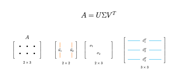
To understand better what is going on, let us focus on recatungular matrix $\boldsymbol{A} \in \mathbb{R}^{3 \times 2}$. This matrix can be perceived as a complex linear transformation from $\mathbb{R}^3 \to \mathbb{R}^2$. If we apply this tranformation to a matrix $\mathbf{x} \in \mathbb{R}^3$ it will return a new vector that lives in $\mathbb{R}^2$ space. When we factorize this matrix using SVD, matrix $\boldsymbol{\Sigma} \in \mathbb{R}^{3 \times 2}$ lives in the same space with the initial matrix $ \boldsymbol{A}$, and it is a diagonal matrix that contains the so-called singular values. Matrices $ \boldsymbol{U} \in \mathbb{R}^{3 \times 3}$ and $\boldsymbol{V} \in \mathbb{R}^{2 \times 2}$ are orthogonal basis in the two spaces that are related to the transformation matrix $\boldsymbol{A}$.

To better grasp the idea behind these matrices, lets think for a moment about the properties of a symmetric matrix which is square matrix where 1) The two sides of the diagonal matrix contains identical entries. That is reflected from the following obvious property: $\boldsymbol{B} = \boldsymbol{B}^{T}$. 2) The eigenvectors of the symmetric matrix are perpendicular to each other. If we store these eigenvectors into a matrix that implies some rotation matrix.

These two properties are important for SVD. Note that our matrix $\boldsymbol{A} \in \mathbb{R}^{3 \times 2}$ is rectangular. However, matrices $\boldsymbol{A}\boldsymbol{A}^{T} \in \mathbb{R}^{2 \times 2}$ (can be denoted as $S_L$) and $\boldsymbol{A}^{T}\boldsymbol{A} \in \mathbb{R}^{3 \times 3}$ ($S_R$) are always symmetric. Here you can see the whole process of SVD:

Visualization of SVD

The visualization of these matrices is shown below (adapted from Wikipedia). We can see that the matrix $\boldsymbol{\Sigma}$ has a diagonal part (which can have zero and non-zero elements), whereas the rest of the matrix is equal to zero.

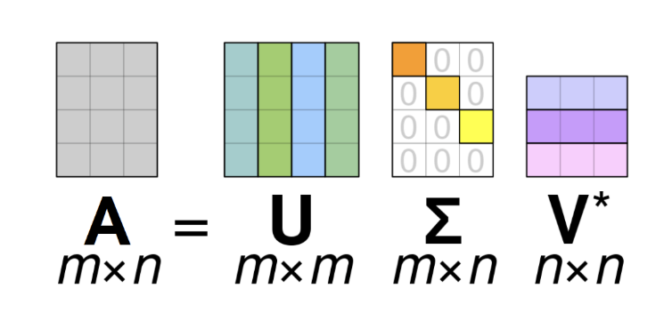
The diagonal elements $\sigma_i = \Sigma_{ii}$ of the matrix $\Sigma$ are called singular values of $\mathbf{A}$.

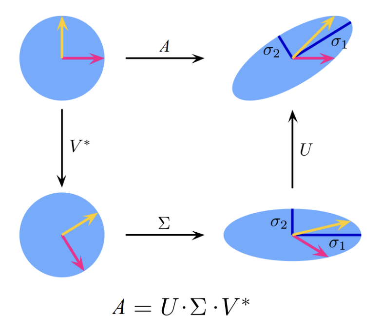
Geometrically, SVD actually performs very simple and intuitive operations. Firstly, the matrix $\mathbf{V}$ performs a rotation in $\mathbb{R}^n$. Next, the matrix $\Sigma$ simply rescales the rotated vectors by a singular value and appends/deletes dimensions to match the dimension $n$ to $m$. Finally, the matrix $\mathbf{U}$ performs a rotation in $\mathbb{R}^m$.

In the case of a real matrix, SVD can be visualized as shown below (adapted from Wikipedia). On the top route, we can see the direct application of a matrix $\mathbf{A}$ on two unit vectors. On the bottom route, we can see the action of each matrix in the SVD. We have used a case of a square matrix, as it is easier to visualize (in general, the matrix $\Sigma$ would add or remove dimensions, depending on the form of the matrix $\mathbf{A}$).

Proof of SVD decomposition

To reason why this decomposition holds can be proven if we perform diagonalization of the matrix $\boldsymbol{A}^{T}\boldsymbol{A}$. This will easily lead to the defition of SVD decomposition.

To prove SVD decompoition, in the general case, where a matrix is not SPD or even square, let’s think of the matrix $\boldsymbol{A}^{T}\boldsymbol{A} \in \mathbb{R}^{m \times m}$ with $\boldsymbol{A} \in \mathbb{R}^{n \times m}$. Let’s start by assuming that matrices $\boldsymbol{A}^T$ and $\boldsymbol{A}$ can be decomposed using SVD. Then, since $\boldsymbol{A}^T\boldsymbol{A}$ is a symmetric and square we can perform eigendecomposition and decompose it in matrix $\boldsymbol{V}$ that contains the eigenvectors and $\boldsymbol{\Sigma}^{T}\boldsymbol{\Sigma}$ that contains the eigevalues which are denoted as $\sigma_{i}^{2}$. That can be seen from the following:

\[\boldsymbol{A}^{\top}\boldsymbol{A} = (\boldsymbol{U}\boldsymbol{\Sigma}\boldsymbol{V}^{\top})^{\top}(\boldsymbol{U}\boldsymbol{\Sigma}\boldsymbol{V}^{\top}) = \boldsymbol{V}\boldsymbol{\Sigma}^{\top}\boldsymbol{U}^{\top}\boldsymbol{U}\boldsymbol{\Sigma}\boldsymbol{V}^{\top} = \boldsymbol{V}\boldsymbol{\Sigma}^T\boldsymbol{\Sigma}\boldsymbol{V}^{\top}\]

Then each column vector $\mathbf{v}_j$ of matrix $\boldsymbol{V}$ is an eigenvector and thus it holds:

\[\boldsymbol{A}^{T}\boldsymbol{A} \cdot \mathbf{v}_j = \sigma_{j}^{2} \mathbf{v}_j\]

Then, if we apply matrix $\boldsymbol{A}$ in both sides of the equation we can end-up having something like as follows:

\[\boldsymbol{A} \boldsymbol{A}^{T} \boldsymbol{A} \cdot \mathbf{v}_j = \sigma_{j}^{2} \boldsymbol{A} \mathbf{v}_j\]

That shows that $\mathbf{u}_j = \boldsymbol{A} \mathbf{v}_j $ is an eigenvector of matrix $\boldsymbol{A} \boldsymbol{A}^{T}$ or we normalize by dividing with $\frac{1}{\sigma_j}$ we end up having the following equation:

\[\boldsymbol{A} \cdot \mathbf{v}_j = \sigma_{j} \mathbf{u}_j\]

Thus, it holds that $\boldsymbol{A} \boldsymbol{V} = \boldsymbol{U} \boldsymbol{\Sigma}$. The final step is to multiply with $\boldsymbol{V}^{-1}$ in both sides and we are finally get

\[\boldsymbol{A} = \boldsymbol{U} \boldsymbol{\Sigma} \boldsymbol{V}^{-1} = \boldsymbol{U} \boldsymbol{\Sigma} \boldsymbol{V}^{T}\]

Dimensionality Reduction with Principal Component Analysis

So far we saw multiple ways to describe data that are stored in a matrix $\boldsymbol{A} \in \mathbf{m \times n}$. We learn about how to compute determinants and the trace of a matrix. We saw also how to perform an eigen-analysis of the matrix and what is the geometric interpretation of it. We examine how to diagonalize a matrix and how to perform decomposition for rectangular matrices using Singular value decomposition (SVD).

Principle component analysis

We will start the explanation of PCA with a simple intuitive example that I like to use when explaining this method.

Conceptually the way that PCA works reminiscence the way that the photography works in the physical space of three dimensions.

Imagine the following setup: there are a group of individuals in the physical world of three dimensions $(x, y, z)$, that represents the coordinates or width, length and height. We want to collect images in such as way that we will represent perfectly all these individuals in the scene (to be able to recognize them all). One option since our problem lives in 3D would be to collect data from three different axis. However, in practice that is not necessary and what a photographer does is to find the perfect angle in 3D space where he can perfectly capture the ideal information for all the subjects in the scene. In the same spirit, we can perceive PCA as finding a new angle to capture our data which better characterize the initial information from our data.

This proper angle is an efficient point of view of observing the data. It can be perceived also as the proper basis that we project the data where we do not need all the dimensions to efficiently describe our data and datasets.

Now the intuition sounds sweet, however, how this is done in practice?

In Principle component analysis (PCA) we are interested in finding projections of the initial data $\mathbf{x}_n \in \mathbb{R}^{D}$ denoted as $\mathbf{\tilde{x}}_n \in \mathbb{R}^{D’}$ which are as close as possible to the original point but at the same time lives in a dimensionality and is lower than the initial one $D’ \ll D$. See that this is exactly what we intended to find by calculating eigenvectors.

Usually, the setup is the following: we do have access to a dataset $\mathcal{D} = \{ \mathbf{x}_1, \mathbf{x}_2, …, \mathbf{x}_n \} \in \mathbb{R}^{N \times D}$ with $N$ to be the number of instances and $D$ the dimensionality of each feature and we can re-write:

\[\boldsymbol{D} = \begin{bmatrix} | & | & & | \\ x_1 & x_2 & \cdots & x_n \\ | & | & & | \end{bmatrix} \in \mathbb{R}^{D \times N}\]

Note that this is a column matrix, meaning that each vector is represented as a column, but sometimes we can have also row-matrix. The same process can be applied in both cases, it is just that perspective changes a bit.

With matrix $\boldsymbol{S}$ to be the data covariance matrix:

\[\boldsymbol{S} = \frac{1}{N}\sum_{i=1} ^N \mathbf{x}_n \mathbf{x}_n^T \in \mathbb{R}^{D \times D}\]

Then in PCA we assume that there is a low dimension representation that is characterized by projection matrix $\boldsymbol{\mathcal{B}} = [ \mathbf{b}_1, \mathbf{b}_2, \cdots, \mathbf{b}_D’ ] \in \mathbb{R}^{D \times D’}$ where you can project each instance $\mathbf{x}_n$ as:

\[\mathbf{z}_n = \boldsymbol{B}^{T} \mathbf{x}_n \in \mathbb{R}^{D'}\]

so we project the data in lower dimensionality $D’ \ll D$

Our target is to find the projection matrix $\boldsymbol{\mathcal{B}}$ that maps the original data with minimal compression loss while keeps the data information intact. In the below sections we will analyze two approaches to find this projection matrix. The approach we will discuss aims at finding the direction that maximizes the variance, while other perspectives try to minimize the reconstruction loss.

First perspective: maximizing the variance

Each vector $[ \mathbf{b}_1, \mathbf{b}_2, \cdots, \mathbf{b}_D’ ] \in \mathbb{R}^{D \times D’}$ projects the initial data into a new coordinate space. The total amount of dimensions is $D’$ and this is a hyperparameter that we usually need to decide or to figure out which dimensionality is more suitable for the problem in hand.

What we can also do here is to sort these projections in such a way that that the first projection leads to the direction with the maximum variance and so on for the rest of the projections. If the dimensionality of the initial data is $D$ then we can find initially $D$ new projections that the variance is maximized and sorted in descending order. Thus, we will need to find these projection vectors that lead to directions where the variance of the data is sorted in this way.

Initially, we start by trying to find the projection vector $\mathbf{b}_1 \in \mathbb{R}^{D}$ that maximizes the variance of the projected data. Usually, in PCA, we make the assumption that the data are centered around mean since the variance is not affected by this mean. That signifies that even if the data are not centered around the mean, if we subtract the mean and center the data, the variance is the same. Thus, we can compute the variance of the first coordinate as:

\[V_1 = \mathbb{V}[z_1] = \frac{1}{N}\sum_{i=1}^{N}z_{1n}^{2}\]

where $z_{1n} = \mathbf{b}_{1}^{T} \mathbf{x}_n$ is the first coordinate that corresponds to the projection of $\mathbf{x}_n$ onto the one-dimensional space spanned by vector $\mathbf{b}_1$. Thus, we can compute the total variance for this dimension based on the input data $\mathcal{D} = \{ \mathbf{x}_1, \mathbf{x}_2, …, \mathbf{x}_n \} \in \mathbb{R}^{N \times D}$:

\[V_1 = \frac{1}{N} \sum_{n=1}^{N} (b_1^\top x_n)^2 = \frac{1}{N} \sum_{n=1}^{N} b_1^\top x_n x_n^\top b_1\] \[= \boldsymbol{b}_1^\top \left( \frac{1}{N} \sum_{n=1}^{N} x_n x_n^\top \right) \boldsymbol{b}_1 = \boldsymbol{b}_1^\top S \boldsymbol{b}_1 .\]

We have expanded the variance and reach to the final expression by using the property that dot product is symmetric. Moreover, we have already defined everything in the parenthesis to be the data covariance:

\[\boldsymbol{S} = \frac{1}{N}\sum_{i=1} ^N \mathbf{x}_n \mathbf{x}_n^T \in \mathbb{R}^{D \times D}\]

To make things easy, in our search for the direction that maximizes the variance, we can assume that the magnitude of this vector is normalized to be equal to one, thus: $||\mathbf{b}_1|| = 1$ since what we care about is the direction and not the length of the vector.

Since we want to find the optimal vector $\mathbf{b}_1 \in \mathbb{R}^{D}$ that maximizes the variance after the projection of the data in hand in this direction that opens the gate for constraint optimization techniques like Lagrangian multipliers:

\[\max_{\boldsymbol{b}_1} \; \boldsymbol{b}_1^{\top} S \boldsymbol{b}_1\] \[\text{subject to } \|\boldsymbol{b}_1\|^2 = 1.\]

This is an equality constraint optimization problem, so we can introduce the following Lagrangian:

\[\mathcal{L} = \boldsymbol{b}_1^\top S \boldsymbol{b}_1 + \lambda_1 (1 - b_1^\top \boldsymbol{b}_1)\]

The recipe for Lagrangian constraint optimization is to find the partial derivatives with respect to $b_{1} $ and $\lambda_{1}$ which leads to the following outcome:

\[\boldsymbol{S}\boldsymbol{b}_1 = \lambda_{1} \boldsymbol{b}_1\]

It is obvious that by computing the partial derivatives we ended up in an equation system that is equal to eigen-decomposition and vector $b_{1}$ is an eigenvector while parameter $\lambda_{1}$ is an eigenvalue. Now, if we dig further we do have the following expression:

\[V_1 = \boldsymbol{b}_1^\top S \boldsymbol{b}_1 = \boldsymbol{b}_1^\top \lambda_{1} \boldsymbol{b}_1 = \lambda_{1} \boldsymbol{b}_1^\top \boldsymbol{b}_1 = \lambda_{1}\]

What this equation expresses is that the to maximize the variance of this projection, we need to find the eigenvector with the largest eigenvalue of the data covariance matrix. Then, this vector $ \boldsymbol{b}_1$ is called first principal component.

Once we found the first PC we can subtract this from the data matrix and perform the same process again until we find $M$ principal component vectors. While we will not present here all the details of how this is done, in principle we can have:

\[\boldsymbol{\hat{X}} = \boldsymbol{X} - \sum_{i=1}^{m-1} b_i b_i^{T} \boldsymbol{X} = \boldsymbol{X} - \boldsymbol{B}_{m-1} \boldsymbol{X}\]

The above shows a generalization of how we can subtract the first $m-1$ principal components from our matrix $\boldsymbol{X}$.

We can proceed that way that we can compute $M$ principal components. We can even compute $M = D$ components. Once we compute all of them, we can sort the PC based on their eigenvalue so the variance in the projected coordinate. Finally, we can keep all the coordinates that lead to minimum reduce of the variance in data with the respect to the variance of the initial data.

####Example MNIST embeddings

####How to use SVD for computing PCA in practise

back